Blog

Your blog category

Blog, forEachBatch, Spark, Stream

Simplifying Real-time Data Processing with Spark Streaming’s foreachBatch with working code

Comprehensive guide to implementing a fully operational Streaming Pipeline that can be tailored to your specific needs. In this working example, you will learn how to parameterize the ForEachBatch function. Spark Streaming & foreachBatch Spark Streaming is a powerful tool for processing streaming data. It allows you to process data as it arrives, without having to wait for the entire dataset to be available. This can be very useful for applications that need to respond to changes in data in real time. One of the features of Spark Streaming is the foreachBatch() method. This method allows you to apply a custom function to each batch of data as it arrives. This can be useful for a variety of tasks, such as: The foreachBatch() method is a powerful tool that can be used to extend the capabilities of Spark Streaming. In this blog post, we will take a closer look at how to use foreachBatch(). Introducing foreachBatch: foreachBatch is a method provided by Spark Streaming that allows developers to apply arbitrary operations on the output of a streaming query. It acts as a bridge between the streaming world and the structured world of DataFrames and Datasets. This means that we can leverage the rich functionality of Spark’s structured APIs to process real-time data efficiently. The Power of foreachBatch: The foreachBatch operation enables developers to perform batch-like operations on streaming data. Instead of processing each individual record, which can be inefficient, foreachBatch processes the data in micro-batches, offering better performance and resource utilization. This approach also provides the flexibility to leverage the full power of Spark’s DataFrames, including various transformations and aggregations, to perform complex computations on streaming data. Implementing foreachBatch: To use foreachBatch, you need to define a function that takes two arguments: the batch identifier and the DataFrame representing the micro-batch of data. Inside this function, you can apply any transformations or computations required on the streaming data. You can use Spark’s SQL, DataFrame, or Dataset APIs to manipulate the data and write the results to any external systems, such as databases or file systems. Benefits of foreachBatch: Code & Setup Here’s how we can use foreachBatch to achieve this: ∘ Define parameters for the job ∘ Create a Streaming source ∘ Define custom processing logic and parameters ∘ Create an instance of forEachBatchProcessor Class with the parameters ∘ Orchestrate the job ∘ Look at the output table ∘ Clean Up Define parameters for the job target_table_name = “for_each_batch_paramerterize” check_point_location = f”/tmp/delta/{target_table_name}/_checkpoints/” dedupe_colum_name =”hash” Create a Streaming source We will create a synthetic dataset. generated_df = ( spark.readStream .format(“rate”) .option(“numPartitions”, 4) .option(“rowsPerSecond”, 1 * 1000) .load() .selectExpr( “md5( CAST (value AS STRING) ) as md5″ ,”value” ,”value%1000000 as hash” ) ) Define custom processing logic and parameters class forEachBatchProcessor: def __init__(self, dedupe_column: str, filter_criteria:str, passed_value: int): self.dedupe_column = dedupe_column self.filter_criteria = filter_criteria self.passed_value = passed_value def print_attributes(self): attributes = vars(self) print( “\n”.join([f”{attr}: {value}” for attr, value in attributes.items()]) ) def make_changes_using_the_micro_batch(self, microBatchOutputDF, batchId: int): self.print_attributes() print(f”Processing batchId: {batchId}”) # Your processing logic using the parameter view_name = f”updates_for_batchId_{batchId}” microBatchOutputDF.createOrReplaceTempView(view_name) sql_logic = f””” SELECT * ,{self.passed_value} as passed_value ,{batchId} as batch_id FROM ( SELECT * ,rank() over(partition by {self.dedupe_column} order by value desc) as dedupe FROM {view_name} WHERE {self.filter_criteria} ) WHERE dedupe =1 “”” print(f”Processing sql_logic: {sql_logic}”) to_be_written_df = microBatchOutputDF.sparkSession.sql(sql_logic).drop(“dedupe”) to_be_written_df.write.mode(“append”).saveAsTable(target_table_name) Create an instance of forEachBatchProcessor Class with the parameters instantiateForEachBatchProcessor = forEachBatchProcessor( dedupe_column = dedupe_colum_name, filter_criteria = “1=1”, passed_value = 3 ) Orchestrate the job ( generated_df .writeStream #.trigger(availableNow=True) .trigger(processingTime=’10 seconds’) .option(“checkpointLocation”, check_point_location) .option(“queryName”, “ParameterizeForEachBatch”) .foreachBatch(instantiateForEachBatchProcessor.make_changes_using_the_micro_batch) .start() ) Look at the output table display(spark.read.table(target_table_name)) Clean Up spark.sql(f””” DROP TABLE IF EXISTS {target_table_name} “””) dbutils.fs.rm(check_point_location,True) Conclusion: Apache Spark Streaming’s foreachBatch operation is a powerful tool for simplifying real-time data processing. By bridging the gap between the streaming and structured worlds, it enables developers to perform batch-like operations on streaming data efficiently. Leveraging the rich functionality of Spark’s DataFrames, foreachBatch empowers users to process and analyze real-time data with ease. Whether you’re performing aggregations, transformations, or writing data to external systems, foreachBatch offers a flexible and scalable solution for real-time streaming applications. Footnote: Thank you for taking the time to read this article. If you found it helpful or enjoyable, please consider clapping to show appreciation and help others discover it. Don’t forget to follow me for more insightful content, and visit my website **CanadianDataGuy.com** for additional resources and information. Your support and feedback are essential to me, and I appreciate your engagement with my work. Download the code I want to emphasize that my blog posts are designed to be practical resources that you can readily use in your own environments. By providing code examples with careful attention to best practices, I aim to simplify the implementation of real-time data processing solutions. I encourage you to explore the blog, copy the code snippets, and adapt them to your specific needs. With these resources, you’ll be equipped to accelerate your development process and unlock the power of Spark Streaming. Dive in, leverage the code, and start building your real-time data processing pipelines with confidence! Go Build! Canadian Data Guy!

Blog, Delta

Delta vs. Parquet: A Deep Dive into Big Data Storage Solutions

Unlocking the intricacies of big data storage solutions is pivotal in today’s data-driven landscape. As organizations grapple with vast amounts of data, choosing between storage formats like Delta and Parquet becomes crucial. Diving deep into their technical nuances, this article highlights why Delta is emerging as the preferred choice for many. From ACID transactions to schema evolution, discover the game-changing features that set Delta apart in the competitive world of data storage. 1. Introduction to Delta and Parquet Parquet: An open-source columnar storage format developed under the Apache Software Foundation. It is designed to be compatible with a wide variety of data processing tools in the Hadoop ecosystem. Delta: Delta Lake is more than just a file format; it’s a storage layer that brings ACID transactions to big data workloads on top of Spark. 2. Technical Differences a. ACID Transactions: b. Schema Evolution: c. Time Travel: d. Storage Efficiency: e. Merge, Update, and Delete: 3. Performance Insights 4. Compatibility and Ecosystem 5. The Verdict While Parquet is a robust columnar storage format that has served the big data community well, Delta brings in features that cater to the evolving needs of data engineering and data science teams. Its emphasis on transactional integrity, combined with advanced optimizations, positions Delta as a formidable player in the big data storage arena.

Best Practices, Blog

How to Cut Your Data Processing Costs by 30% with Graviton

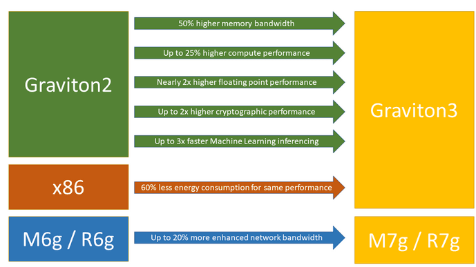
What is AWS Graviton ? AWS Graviton is a family of Arm-based processors that are designed by AWS to provide cost-effective and high-performance computing for cloud workloads. Graviton processors are built using 64-bit Arm, which are optimized for power efficiency and performance. They offer a more cost-effective alternative to traditional x86-based processors, making them a popular choice for running a variety of workloads on AWS. With Graviton, you can enjoy lightning-fast data processing speeds while saving money on your infrastructure costs. Plus, Graviton is compatible with all your favorite tools and applications, so you can seamlessly integrate it into your existing workflow. Overall, AWS Graviton offers a flexible and cost-effective alternative to traditional x86-based processors, making it a popular choice for customers who are looking to optimize their cloud computing costs without sacrificing performance or reliability. Cost Savings If you look at the screenshot below, you will find Graviton cheaper than every other series. **Decipher instance name: c6g.xlarge: **C stands for compute series, 6 stands for a series number, g stands for Graviton, and xLarge means 4 vCPU. Compute Intensive (C Series) c6g.xlarge is 12.5% cheaper than the next cheapest instance. General Purpose (M Series) m6g.xlarge is ~12.2% cheaper than the next cheapest instance. Memory Intensive ( R Series) r6g.xlarge is ~12.5% cheaper than the next cheapest instance. This is complicated. Help me choose ? Let me break down the AWS instance series into simple parts. Think about how much memory you get per core, and the price increases as the memory increases. I recommend that customers start with general purpose, get a baseline runtime, and then try different series. The best way to gauge what instance family would work is to identify or categorize if the workload is compute-bound, memory-bound or network bound. Launch of new Graviton 3 series in 2023 Here are some benefits of the new Graviton 3 series; the price is ~10% more expensive Graviton 2. However, it’s still cheaper than the M6 a instance. M6g ($ 0.154) < M7g ($ 0.1632) < M6a ( $0.1728 ) New Graviton3-Based General Purpose (m7g) and Memory-Optimized (r7g) Amazon EC2 Instances | Amazon… *We’ve come a long way since the launch of the m1.small instance in 2006, adding instances with additional memory…*aws.amazon.com Conclusion As you can see, the price saving is at least ~12%, and AWS claims 40% better price performance due to faster processors. Thus, in reality, you should be able to save 12–40% cost savings at least. In my real-world experience, I have seen 20–30% cost savings. Footnote: Thank you for taking the time to read this article. If you found it helpful or enjoyable, please consider clapping to show appreciation and help others discover it. Don’t forget to follow me for more insightful content, and visit my website **CanadianDataGuy.com** for additional resources and information. Your support and feedback are essential to me, and I appreciate your engagement with my work.

Blog

A Productive Life: How to Parallelize Code Execution in Python

Asynchronous programming has become increasingly popular in recent years, especially in web development, where it is used to build high-performance, scalable applications. Python has built-in support for asynchronous programming through the asyncio module, which provides a powerful framework for writing asynchronous code. In this blog post, we will explore the asyncio module in Python 3.10 and learn how to run tasks in parallel using the new features introduced in this version. We will explore 3 examples here: Example 1: Asyncio Tasks / create_task() In asyncio, a task is a unit of work that is scheduled to run on the event loop. Tasks are created from coroutines, which are functions that are defined using the async def syntax and that can suspend their execution using the await keyword. To create a task, we use the asyncio.create_task() function, which takes a coroutine as its argument and returns a Task object. We can then schedule the task to run on the event loop using the await keyword. Here’s an example: import asyncio async def function_which_will_run_in_parallel(): # Add what you want to do here print(‘function_which_will_run_in_parallel completed’) # Orchestrate function async def main(): task = asyncio.create_task(function_which_will_run_in_parallel()) await task asyncio.run(main()) In this example, we define a simple function_which_will_run_in_parallel() that waits for one second and then prints a message. In the main() function, we create a Task object using asyncio.create_task() and pass it the function. We then await the completion of the task using await task. When we run the main() using asyncio.run(), the Task object is created and scheduled on the event loop, which runs the function_which_will_run_in_parallel() function asynchronously. Once the function_which_will_run_in_parallel() function is complete, the Task object is marked as done, and the program exits. Example 2: Running Tasks in Parallel In asyncio, we can run tasks in parallel using the asyncio.gather() function. This function takes one or more coroutines/functions as its arguments and returns a list of their results. Here’s an example: import asyncio async def coroutine1(): await asyncio.sleep(1) return ‘Coroutine 1 completed’ async def coroutine2(): await asyncio.sleep(2) return ‘Coroutine 2 completed’ async def main(): results = await asyncio.gather(coroutine1(), coroutine2()) print(results) asyncio.run(main()) In this example, we define two coroutines, coroutine1() and coroutine2(), that wait for one and two seconds, respectively, before returning a message. In the main() coroutine function, we use the asyncio.gather() function to run the two coroutines in parallel. We pass coroutine1() and coroutine2() as its arguments and use await to wait for both coroutines to complete. When both coroutines are complete, the asyncio.gather() function returns a list of their results, which we print to the console. Example 3: Running tasks in parallel with a loop In this example, we define an asynchronous coroutine function fetch() that uses the aiohttp library to download the contents of a given URL. We then define the main() coroutine function that creates a list of URLs to download and uses asyncio.create_task() to create a task for each URL. We then use asyncio.gather() to wait for all tasks to complete and return their results. The async with aiohttp.ClientSession() context manager is used to create a session object that can be reused across multiple requests, which can improve performance. When we run the main() coroutine using asyncio.run(), it concurrently downloads the web pages from the list of URLs, and prints the number of bytes downloaded from each URL. This is just a simple example, but it demonstrates how asyncio can be used to concurrently perform I/O-bound tasks such as web page downloads. import asyncio import aiohttp async def fetch(session, url): async with session.get(url) as response: return await response.text() async def main(): urls = [ ‘https://example.com’, ‘https://google.com’, ‘https://facebook.com’, ‘https://twitter.com’, ‘https://linkedin.com’, ] async with aiohttp.ClientSession() as session: tasks = [asyncio.create_task(fetch(session, url)) for url in urls] results = await asyncio.gather(*tasks) for url, result in zip(urls, results): print(f”Downloaded {len(result)} bytes from {url}”) asyncio.run(main()) Conclusion Asyncio is a powerful framework for writing asynchronous code in Python, and with the new features introduced in Python 3.10, it has become even easier to run tasks in parallel. In this blog post, we learned how to create tasks using asyncio.create_task() and how to run tasks in parallel using `asyncio.gather() Footnote: Thank you for taking the time to read this article. If you found it helpful or enjoyable, please consider clapping to show appreciation and help others discover it. Don’t forget to follow me for more insightful content, and visit my website **CanadianDataGuy.com** for additional resources and information. Your support and feedback are essential to me, and I appreciate your engagement with my work.

Blog, Delta, Spark

What is inside a Spark Streaming Checkpoint

Spark is a distributed computing framework that allows for processing large datasets in parallel across a cluster of computers. When running a Spark job, it is not uncommon to encounter failures due to various issues such as network or hardware failures, software bugs, or even insufficient memory. One way to address these issues is to re-run the entire job from the beginning, which can be time-consuming and inefficient. To mitigate this problem, Spark provides a mechanism called check-pointing. Why do we even need a checkpoint? Someone needs to remember what was done before or what was processed before, or what we know so far. All this information needs to be stored somewhere. The place where this is stored is called a Checkpoint. How does checkpoint work? Think of it as a 3 step process: Checkpoints store the current offsets and state values (e.g. aggregate values) for your stream. Checkpoints are stream specific, so each should be set to its own location. This is an advanced blog and should be read with the expectation of familiarizing and not understanding. Read this and bookmark it; once you come across a situation where you need to dig into the checkpoint, this blog will come in handy. What is inside a checkpoint folder? It will have 3 folders inside it and a metadata file: What is inside the Offsets file? The easiest way to think about it is that once we start processing a micro-batch of data. We need to store an upper bound mark and a lower bound mark of the data. This mark could be called an offset. Think if you a measuring something with a scale and you need to log the reading. This reading, aka the offset, we will store in the offsets file. Different sources like Kafka, Kinesis, Delta, etc., all have different ways of defining offsets, but conceptually they are the same. For this blog, let’s concentrate on Delta as a streaming source. This stores the stream-id, which is generated when the stream starts and remains the same throughout the life of the checkpoint. Commits These files are generated only when the micro-batch succeeds. Offsets are generated at the start of the micro-batch. If the offset did not have a corresponding commit, a failure happened when processing that offset. In an ideal scenario, the number of commit files equals the number of offset files. However, when they are not equal, the next Spark Streaming knows where to start because it’s stored in the offset file, which did not have a corresponding commit. Furthermore, watermarking information would be found here. State Store This folder only has data in the case of Stateful Streaming, where the State is stored on disk for resiliency purposes. Thus when failures happen, the state can be recovered from here. References Please spare some time to look at the below to help absorb the above content further. Footnote: Thank you for taking the time to read this article. If you found it helpful or enjoyable, please consider clapping to show appreciation and help others discover it. Don’t forget to follow me for more insightful content, and visit my website CanadianDataGuy.com for additional resources and information. Your support and feedback are essential to me, and I appreciate your engagement with my work.

Blog, Databricks

How to get the Job ID, Run ID & Start Time for a Databricks Job with working code

It’s crucial to monitor task parameter variables such as job_id, run_id, and start_time while running ELT jobs. These system-generated values can be saved or printed for future reference. Please refer below to find the comprehensive list of supported parameters. This is a simple 2-step process: Step 1: Pass the parameters Step 2: Get/Fetch and print the values print(f””” job_id: {dbutils.widgets.get(‘job_id’)} run_id: {dbutils.widgets.get(‘run_id’)} parent_run_id: {dbutils.widgets.get(‘parent_run_id’)} task_key: {dbutils.widgets.get(‘task_key’)} “””) Next step, when you run the job; you should see an output like this Advanced & quicker method to implement Add the following boilerplate code on top of the notebook. It will capture whole context information instead, and you can parse whatever information is helpful to you. The below is code based and attributes are subject to change without notice import json, pprintdict_job_run_metadata = json.loads(dbutils.notebook.entry_point.getDbutils().notebook().getContext().toJson())print(f”’ currentRunId: {dict_job_run_metadata[‘currentRunId’]} jobGroup: {dict_job_run_metadata[‘jobGroup’]} ”’)# Pretty print the dictionarypprint.pprint(dict_job_run_metadata) Footnote Thank you for taking the time to read this article. If you found it helpful or enjoyable, please clapping to show appreciation and help others discover it. Don’t forget to follow me for more insightful content, and visit my website CanadianDataGuy.com for additional resources and information. Your support and feedback are essential to me, and I appreciate your engagement with my work.

Blog, Databricks, Spark, Stream

How to write your first Spark Stream Batch Join with working code

When I started learning about Spark Streaming, I could not find enough code/material which could kick-start my journey and build my confidence. I wrote this blog to fill this gap which could help beginners understand how simple streaming is and build their first application. In this blog, I will explain most things by first principles to increase your understanding and confidence and you walk away with code for your first Streaming application. Scenario: Let’s assume we have a streaming source with data arriving all the time. We want to add more attributes from another table( Think lookup table/ dimension table). Thus we will stream the data and join with the lookup table via Stream-Batch join. The result would be written as a Delta table, which could be used downstream for analytics or streaming. Imports & Parameters from pyspark.sql import functions as Ffrom faker import Fakerimport uuid# define schema name and where should the table be storedschema_name = “test_streaming_joins”schema_storage_location = “/tmp/CHOOSE_A_PERMANENT_LOCATION/”# Please download this file from https://simplemaps.com/data/us-zips then download and place it at a location of your choice and then change the value for the variable belowstatic_table_csv_file = “/FileStore/jitesh.soni/data/us_zip_code_and_its_attributes.csv”# Static table specificationstatic_table_name = “static_zip_codes”# Target Stareaming Table specificationtarget_table_name = “joined_datasets”# Recommend you to keep the checkpoint next to the Delta table so that you do have to notion about where the checkpoint ischeckpoint_location = f”{schema_storage_location}/{target_table_name}/_checkpoints/”Create Target Database create_schema_sql = f””” CREATE SCHEMA IF NOT EXISTS {schema_name} COMMENT ‘This is {schema_name} schema’ LOCATION ‘{schema_storage_location}’ WITH DBPROPERTIES ( Owner=’Jitesh’); “””print(f”create_schema_sql: {create_schema_sql}”) Generate Static Or a lookup Dataset We will use a public dataset source with attributes about a zip code. This could be any other static source or a Delta table being updated in parallel. Note: If you pick a static source and start streaming, Spark Streaming will only read it once. If you have a few updates to the static source, you will have to restart the Spark Stream so it rereads the static source. Meanwhile, if you have the Delta table as a source, then Spark Streaming will identify the update automatically, and nothing extra needs to be done. csv_df = ( spark.read.option(“header”, True) .option(“inferSchema”, True) .csv(static_table_csv_file))display(csv_df)csv_df.write.saveAsTable(f”{schema_name}.{static_table_name}”) Next, we will Z-order the table on the key, which would be used in joins. This will help Spark Streaming do efficient joins because the Delta table is sorted by join key with statistics about which file contains which key value. spark.sql( f””” OPTIMIZE {schema_name}.{static_table_name} ZORDER BY (zip); “””) Generate Streaming Dataset We will generate a Streaming dataset using the Faker library. In the below code, we will define a few user-defined functions. fake = Faker()fake_id = F.udf(lambda: str(uuid.uuid4()))fake_firstname = F.udf(fake.first_name)fake_lastname = F.udf(fake.last_name)fake_email = F.udf(fake.ascii_company_email)# fake_date = F.udf(lambda:fake.date_time_this_month().strftime(“%Y-%m-%d %H:%M:%S”))fake_address = F.udf(fake.address)fake_zipcode = F.udf(fake.zipcode) Now, we will use spark.readStream.format(“rate”) to generate data at your desired rate. streaming_df = ( spark.readStream.format(“rate”) .option(“numPartitions”, 10) .option(“rowsPerSecond”, 1 * 1000) .load() .withColumn(“fake_id”, fake_id()) .withColumn(“fake_firstname”, fake_firstname()) .withColumn(“fake_lastname”, fake_lastname()) .withColumn(“fake_email”, fake_email()) .withColumn(“fake_address”, fake_address()) .withColumn(“fake_zipcode”, fake_zipcode()))# You can uncomment the below display command to check if the code in this cell works# display(streaming_df) Stream- Static Join or Stream -Delta Join Structured Streaming supports joins (inner join and left join) between a streaming and a static DataFrame or a Delta Table. However, a few types of stream-static outer Joins are not supported yet. lookup_delta_df = spark.read.table(static_table_name)joined_streaming_df = streaming_df.join( lookup_delta_df, streaming_df[“fake_zipcode”] == lookup_delta_df[“zip”], “left_outer”,).drop(“fake_zipcode”)# display(joined_streaming_df) Orchestrate the pipeline and write Spark Stream to Delta Table Some Tips: ( joined_streaming_df.writeStream # .trigger(availableNow=True) .queryName(“do_a_stream_join_with_the_delta_table”) .option(“checkpointLocation”, checkpoint_location) .format(“delta”) .toTable(f”{schema_name}.{target_table_name}”)) Download the code Footnote: Thank you for taking the time to read this article. If you found it helpful or enjoyable, please consider clapping to show appreciation and help others discover it. Don’t forget to follow me for more insightful content, and visit my website CanadianDataGuy.com for additional resources and information. Your support and feedback are essential to me, and I appreciate your engagement with my work.

Blog, Delta, Spark, Stream

How to upgrade your Spark Stream application with a new checkpoint With working code

Sometimes in life, we need to make breaking changes which require us to create a new checkpoint. Some example scenarios: There could be plenty of scenarios where you want to control precisely which data(Kafka offsets) need to be processed. Not every scenario requires a new checkpoint. Here is a list of things you can change without requiring a new checkpoint. This blog helps you understand how to handle a scenario where a new checkpoint is unavoidable. Kafka Basics: Topics, partition & offset Kafka Cluster has Topics: Topics are a way to organize messages. Each topic has a name that is unique across the entire Kafka cluster. Messages are sent to and read from specific topics. In other words, producers write data on a topic, and consumers read data from the topic. Topics have Partitions, and data/messages are distributed across partitions. Every message belongs to a single partition. Partition has messages, each with a unique sequential identifier within the partition called the Offset. What is the takeaway here? We must identify what offset has already been processed for each partition, and this information can be found inside the checkpoint. What information is inside the checkpoint? Under the checkpoint folder, there are four subfolders: How to fetch information about Offset & Partition from the Checkpoint folder? List the files at the checkpoint location; we are looking for the offsets folder. checkpoint_location= “/checkpoint_location/checkpoint_for_kafka_to_delta”dbutils.fs.ls(checkpoint_location)dbutils.fs.ls(f”{checkpoint_location}/”) Next, we will list the files under the commits folder and identify the most recent commits. dbutils.fs.ls(checkpoint_location)dbutils.fs.ls(f”{checkpoint_location}/commits”) /checkpoint_location/checkpoint_for_kafka_to_delta/commits/0/checkpoint_location/checkpoint_for_kafka_to_delta/commits/1/checkpoint_location/checkpoint_for_kafka_to_delta/commits/2 Once we identify the last commits file number; we will open the equivalent offsets file. In this example, we can see the latest commits is “2”. Now let’s view the contents of the offsets file. #%fs head {FILL_THE_EXACT_PATH_OF_THE_FILE_WHICH_NEEDS_TO_BE_VIEWED}%fs head /checkpoint_location/checkpoint_for_kafka_to_delta/offsets/2{“batchWatermarkMs”:0,”batchTimestampMs”:1674623173851,”conf”:{“spark.sql.streaming.stateStore.providerClass”:”org.apache.spark.sql.execution.streaming.state.HDFSBackedStateStoreProvider”,”spark.sql.streaming.join.stateFormatVersion”:”2″,”spark.sql.streaming.stateStore.compression.codec”:”lz4″,”spark.sql.streaming.stateStore.rocksdb.formatVersion”:”5″,”spark.sql.streaming.statefulOperator.useStrictDistribution”:”true”,”spark.sql.streaming.flatMapGroupsWithState.stateFormatVersion”:”2″,”spark.sql.streaming.multipleWatermarkPolicy”:”min”,”spark.sql.streaming.aggregation.stateFormatVersion”:”2″,”spark.sql.shuffle.partitions”:”200″}}{“topic_name_from_kafka”:{“0”:400000, “1”:300000}} The information of interest is in the end. This has the topic name and offset per partition. {“topic_name_from_kafka”:{“0”:400000, “1”:300000}} Now the easy part: Use Spark to start reading Kafka from a particular Offset Spark Streaming starts read stream by default with the latest offset. However, it provides a parameter “startingOffsets” to select a custom starting point. startingOffsets = “””{“topic_name_from_kafka”:{“0”:400000, “1”:300000}}”””kafka_stream = (spark.readStream .format(“kafka”) .option(“kafka.bootstrap.servers”, kafka_bootstrap_servers_plaintext ) .option(“subscribe”, topic ) .option(“startingOffsets”, startingOffsets ) .load())display(kafka_stream) And we are Done!!. Recommend parameterizing your code so that “startingOffsets” can be passed as a parameter. Footnote: Thank you for taking the time to read this article. If you found it helpful or enjoyable, please consider clapping to show appreciation and help others discover it. Don’t forget to follow me for more insightful content, and visit my website CanadianDataGuy.com for additional resources and information. Your support and feedback are essential to me, and I appreciate your engagement with my work.

Blog, Delta, Delta Live Tables

How to parameterize Delta Live Tables and import reusable functions with working code

This blog will discuss passing custom parameters to a Delta Live Tables (DLT) pipeline. Furthermore, we will discuss importing functions defined in other files or locations. You can import files from the current directory or a specified location using sys.path.append(). Update: As of December 2022, you can directly import files if the reusable_functions.py file exists in the same repository by just using the import command, which is the preferred approach. However, in case these reusable_functions.py file exists outside the repository, you can take the sys.path.append() approach mentioned below. Overall, this a 4-step process: 1. Create a reusable_functions.py file Create a reusable function in a Python File (not Notebook), so we can import it later. Let’s call the file ‘reusable_functions.py’ below and place it in a path. Please make sure to note the absolute path of the folder where this file will be placed. from pyspark.sql import DataFramefrom pyspark.sql.functions import current_timestamp, current_datedef append_ingestion_columns(_df: DataFrame): return _df.withColumn(“ingestion_timestamp”, current_timestamp()).withColumn( “ingestion_date”, current_date() ) 2. Add code to receive the DLT parameters The below function is defined with try and except block so that it can work with Notebook as well, where we cannot pass the parameter value from the DLT pipeline from pyspark.sql import SparkSessiondef get_parameter_or_return_default( parameter_name: str = “pipeline.parameter_blah_blah”, default_value: str = “default_value”,) -> str: try: spark = SparkSession.getActiveSession() if spark is not None: parameter = spark.conf.get(parameter_name) else: raise Exception(“No active Spark session found.”) except Exception as e: print(f”Caught Exception: {e}. Using default value for {parameter_name}”) parameter = default_value return parameter In this example, we will pass two parameters: path_to_reusable_functions & parameter_abc. Then we will use the function defined previously to get and set default values for both. path_to_reusable_functions = get_parameter_or_return_default( parameter_name=”pipeline.path_to_reusable_functions”, default_value=”/Workspace/Repos/jitesh.soni@databricks.com/material_for_public_consumption/”,)parameter_abc = get_parameter_or_return_default( parameter_name=”pipeline.parameter_abc”, default_value=”random_default_value”) 3. Append the path to reusable_functions.py file and import the functions in the notebook import sys# Add the path so functions could be importedsys.path.append(path_to_reusable_functions)# Attempt the importfrom reusable_functions import append_ingestion_columns Next step, we will define a function to return a DataFrame and the run display command to see the output of the function. This helps one test if the code works without running the DLT pipeline. def static_dataframe(): df_which_we_got_back_after_running_sql = spark.sql( f””” SELECT ‘{path_to_reusable_functions}’ as path_to_reusable_functions ,'{parameter_abc}’ as parameter_abc “”” ) return append_ingestion_columns(df_which_we_got_back_after_running_sql)display(static_dataframe()) At this point, you should be able to run your notebook and validate everything works before we create a DLT pipeline. Next step, we define a DLT table. import dlt@dlt.table(name=”static_table”, comment=”Static table”)def dlt_static_table(): return static_dataframe() 4. Create a DLT pipeline and set/pass parameters At this step, we can create a DLT pipeline via UI, add our custom parameters, and assign them values. The full JSON representation would look something like this, we only care about the configuration section in this JSON. { “id”: “d40fa97a-5b5e-4fe7-9760-b67d78a724a1”, “clusters”: [ { “label”: “default”, “policy_id”: “E06216CAA0000360”, “autoscale”: { “min_workers”: 1, “max_workers”: 2, “mode”: “ENHANCED” } }, { “label”: “maintenance”, “policy_id”: “E06216CAA0000360” } ], “development”: true, “continuous”: false, “channel”: “PREVIEW”, “edition”: “CORE”, “photon”: false, “libraries”: [ { “notebook”: { “path”: “/Repos/jitesh.soni@databricks.com/material_for_public_consumption/notebooks/how_to_parameterize_delta_live_tables_and_import_reusable_functions” } } ], “name”: “how_to_parameterize_delta_live_tables_and_import_reusable_functions”, “storage”: “dbfs:/pipelines/d40fa97a-5b5e-4fe7-9760-b67d78a724a1”, “configuration”: { “pipeline.parameter_abc”: “this_was_passed_from_dlt_config”, “pipeline.path_to_reusable_functions”: “/Workspace/Repos/jitesh.soni@databricks.com/material_for_public_consumption/” }, “target”: “tmp_taget_schema”} Trigger your DLT pipeline. If you have reached so far, you should have an end-to-end DLT pipeline working with parameter passing and imports. *Update | How do you edit these parameters via API or CLI Below are screenshots of how to edit these parameters via CLI. The API solution would be similar. Create a JSON file with the parameters: { “id”: “d40fa97a-5b5e-4fe7-9760-b67d78a724a1”, “name”: “how_to_parameterize_delta_live_tables_and_import_reusable_functions”, “clusters”: [ { “label”: “default”, “policy_id”: “E06216CAA0000360”, “autoscale”: { “min_workers”: 1, “max_workers”: 5, “mode”: “ENHANCED” } }, { “label”: “maintenance”, “policy_id”: “E06216CAA0000360″ } ],”configuration”: { “pipeline.parameter_created_from_jobs_cli”: “this_was_created_from_jobs_cli”, “pipeline.parameter_abc”: “this_was_passed_from_dlt_config_via_job_cli”, “pipeline.path_to_reusable_functions”: “/Workspace/Repos/jitesh.soni@databricks.com/material_for_public_consumption/” }, “libraries”: [ { “notebook”: { “path”: “/Repos/jitesh.soni@databricks.com/material_for_public_consumption/notebooks/how_to_parameterize_delta_live_tables_and_import_reusable_functions” } } ]} Call the Datarbricks CLI to push the changes: Go back to Delta Live Tables UI and the change would have gone through Download the code DLT notebook and Reusable_function.py Footnote: Thank you for taking the time to read this article. If you found it helpful or enjoyable, please consider clapping to show appreciation and help others discover it. Don’t forget to follow me for more insightful content, and visit my website CanadianDataGuy.com for additional resources and information. Your support and feedback are essential to me, and I appreciate your engagement with my work. References Delta Live Tables settings Delta Live Tables settings specify one or more notebooks that implement a pipeline and the parameters specifying how to… docs.databricks.com

Best Practices, Blog, Stream

Spark Streaming Best Practices-A bare minimum checklist for Beginners and Advanced Users

Most good things in life come with a nuance. While learning Streaming a few years ago, I spent hours searching for best practices. However, I would find answers to be complicated to make sense for a beginner’s mind. Thus, I devised a set of best practices that should hold true in almost all scenarios. The below checklist is not ordered, you should aim to check off as many items as you can. Beginners best practices checklist for Spark Streaming: .option(“queryName”, “IngestFromKafka”) (input_stream .select(col(“eventId”).alias(“key”), to_json(struct(col(‘action’), col(‘time’), col(‘processingTime’))).alias(“value”)) .writeStream .format(“kafka”) .option(“kafka.bootstrap.servers”, kafka_bootstrap_servers_plaintext ) .option(“kafka.security.protocol”, “to_be_filled”) .option(“checkpointLocation”, checkpoint_location ) .option(“topic”, topic) .option(“queryName”, “IngestFromKafka”) .start() ) spark.readStream.format(“kinesis”).**option(“streamName”, stream_name) ** Advanced best practices checklist for Spark Streaming: References: Footnote: Thank you for taking the time to read this article. If you found it helpful or enjoyable, please consider clapping to show appreciation and help others discover it. Don’t forget to follow me for more insightful content, and visit my website **CanadianDataGuy.com** for additional resources and information. Your support and feedback are essential to me, and I appreciate your engagement with my work.

Scroll to Top