...

Best Practices

Best Practices, Blog, Spark, Stream

Learnings from the Field: How to Give Your Spark Streaming Jobs a 15x Speed Boost Using the Lesser-Known Parameter

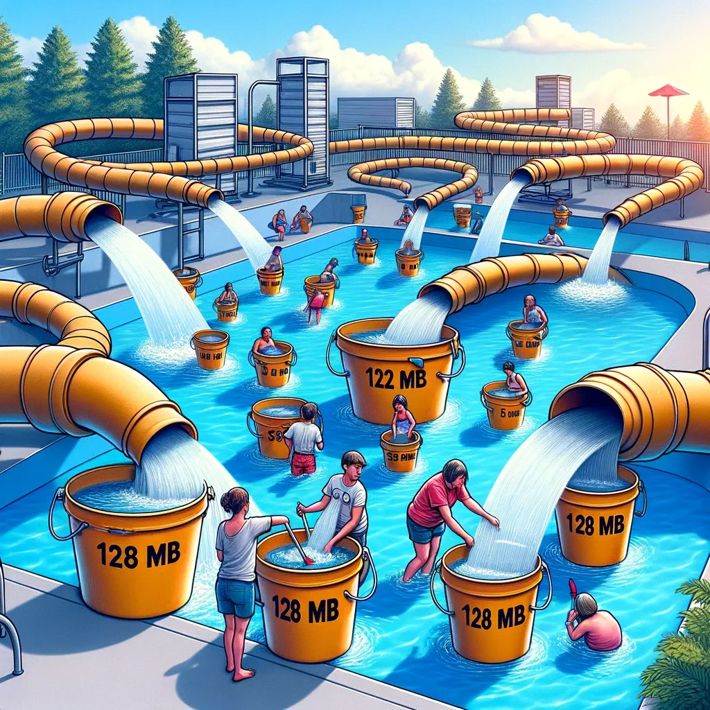
Introduction: In the realm of big data processing, where efficiency and speed are paramount, Apache Spark shines as a potent tool. Yet, the true power of Spark often lies in the nuances of its configuration, particularly in a parameter that might not catch the eye at first glance: spark.sql.files.maxPartitionBytes. This blog unveils how a subtle tweak to this parameter can dramatically amplify the performance of your Spark Streaming jobs, offering up to a 15x speed boost. The Default Behavior — The Large Bucket Dilemma: Imagine you’re at a water park, trying to fill a massive pool using several hoses. Each hose fills a large 128 MB bucket before emptying it into the pool. This is akin to Spark’s default behavior, where each core (or hose) processes data up to 128 MB before moving it further down the pipeline. While this method works, it’s not the most efficient, especially when dealing with numerous smaller files. The large bucket size could lead to slower fill times, underutilizing the hoses and delaying the pool’s completion if you can aquire more hoses(cores). Real-World Implications — The Need for More Buckets: Consider a scenario where a business relies on Spark Streaming for real-time data analysis. They notice the data processing isn’t as swift as expected, despite having ample computational resources. The issue? The oversized 128 MB buckets. With such large buckets, each core is focused on filling its bucket to the brim before contributing to the pool, creating a bottleneck that hampers overall throughput. Adjusting for Performance The Shift to Smaller Buckets: To enhance efficiency, imagine switching to smaller buckets, allowing each hose to fill them more quickly and thus empty more buckets into the pool in the same amount of time. In Spark terms, reducing spark.sql.files.maxPartitionBytes enables the system to create more, smaller data partitions. This adjustment means data can be processed in parallel more effectively, engaging more cores (or hoses) and accelerating the pool-filling process – the data processing task at hand. Understanding the Trade-offs — Finding the Right Bucket Size Opting for smaller buckets increases the number of trips to the pool, akin to Spark managing more partitions, which could introduce overhead from task scheduling and execution. However, too large buckets (or the default setting) might not leverage the full potential of your resources, leading to inefficiencies. The optimal bucket size (partition size) strikes a balance, ensuring each hose (core) contributes effectively without overwhelming the system with overhead. Best Practices — Tuning Your Spark Application: To identify the ideal spark.sql.files.maxPartitionBytes setting, you’ll need to experiment with your specific workload. Monitor the performance impacts of different settings, considering factors like data processing speed, resource utilization, and job completion time. The goal is to maximize parallel processing while minimizing overhead, ensuring that your data processing “water park” operates at peak efficiency. Practical Implications Adjusting spark.sql.files.maxPartitionBytes can have profound effects on the behavior of Spark Streaming jobs: Note: This parameter only applies to file-based sources like an autoloader. Conclusion Adjusting spark.sql.files.maxPartitionBytes is akin to optimizing the bucket size in a massive, collaborative effort to fill a pool. This nuanced configuration can significantly enhance the performance of Spark Streaming jobs, allowing you to fully harness the capabilities of your computational resources. By understanding and fine-tuning this parameter, you can transform your data processing workflow, achieving faster, more efficient results that propel your big data initiatives forward. References and Insights Footnote: Thank you for taking the time to read this article. If you found it helpful or enjoyable, please consider clapping to show appreciation and help others discover it. Don’t forget to follow me for more insightful content, and visit my website CanadianDataGuy.com for additional resources and information. Your support and feedback are essential to me, and I appreciate your engagement with my work.

Best Practices, Blog, forEachBatch, Spark, Stream

Streaming Any File Type with Autoloader in Databricks: A Working Guide

Spark Streaming has emerged as a dominant force as a streaming framework, known for its scalable, high-throughput, and fault-tolerant handling of live data streams. While Spark Streaming and Databricks Autoloader inherently support standard file formats like JSON, CSV, PARQUET, AVRO, TEXT, BINARYFILE, and ORC, their versatility extends far beyond these. This blog post delves into the innovative use of Spark Streaming and Databricks Autoloader for processing file types which are not natively supported. The Process Flow: In the below example is for ROS Bag but the same method could be translated for any other file type. Setting Up the Environment Firstly, we need to prepare our Databricks environment: # Databricks notebook source# MAGIC %pip install bagpydbutils.library.restartPython() We install bagpy, a Python library for ROS bag files, and restart the Python environment to ensure the library is properly loaded.Importing Necessary Libraries Next, we import the required Python libraries: from typing import List, Dictimport boto3import rosbagimport tempfilefrom pyspark.sql.functions import udf, explodefrom pyspark.sql.types import ArrayType, StructType, StructField, IntegerType, LongType, FloatTypefrom pyspark.sql import SparkSession These imports include standard data manipulation tools, AWS S3 access (boto3), ROS bag reading capabilities (rosbag), and necessary PySpark components. Detect new files and file path using Autoloader # Spark streaming setup for ROS bag filess3_data_path = “s3a://one-env/jiteshsoni/Vehicle/”table_name = “rosbag_imu”checkpoint_location = f”/tmp/checkpoint/{table_name}/”stream_using_autoloader_df = (spark.readStream .format(“cloudFiles”) .option(“cloudFiles.format”, “binaryfile”) .option(“cloudFiles.includeExistingFiles”, “true”) .load(s3_data_path) )display(stream_using_autoloader_df)Custom UDF to read & parse any file type The core function extract_rosbag_data reads data from a ROS bag file in an S3 bucket and returns a list of dictionaries containing the extracted data: def extract_rosbag_data(s3_rosbag_path: str) -> List[Dict]: “”” Extracts data from a ROS bag file stored in S3, converting it into a list of dictionaries. Args: s3_rosbag_path (str): The S3 path to the ROS bag file. Returns: List[Dict]: A list of dictionaries with data from the ROS bag. “”” interested_topics = [‘/ublox_trunk/ublox/esfalg’] extracted_data = [] # Extracting the S3 bucket and file key from the provided path bucket_name, s3_file_key = s3_rosbag_path.split(‘/’, 3)[2:4] # Using boto3 to download the ROS bag file into memory s3 = boto3.resource(‘s3’) obj = s3.Object(bucket_name, s3_file_key) file_stream = obj.get()[‘Body’].read() # Storing the downloaded file temporarily with tempfile.NamedTemporaryFile() as temp_file: temp_file.write(file_stream) temp_file.flush() # Reading messages from the ROS bag file with rosbag.Bag(temp_file.name, ‘r’) as bag: for topic, msg, timestamp in bag.read_messages(topics=interested_topics): message_data = {field: getattr(msg, field) for field in msg.__slots__} message_data[‘timestamp’] = timestamp.to_sec() extracted_data.append(message_data) return extracted_data This function uses boto3 to access the S3 bucket, reads the ROS bag file, and extracts the relevant data. At this point, we should test the function before we proceed. For your use case, you want to change this function to read your file type. extract_rosbag_data(s3_rosbag_path= “s3a://bucket_name/jiteshsoni/Vehicle/2023-08-04-16-30-24_63.bag”) Things to note here: In this example, I am downloading the file on the cluster which could be avoided depending if your file reader supports it. Defining the Data Schema Before ingesting data into Spark, define the schema that aligns with the data structure in ROS bags. This is important because Spark needs to know what schema to expect. # Define the schema that matches your ROS bag data structurerosbag_schema = ArrayType(StructType([ StructField(“Alpha”, LongType(), True), StructField(“Beta”, IntegerType(), True), StructField(“Gamma”, IntegerType(), True), StructField(“Delta”, IntegerType(), True), StructField(“Epsilon”, IntegerType(), True), StructField(“Zeta”, IntegerType(), True), StructField(“Eta”, IntegerType(), True), StructField(“Theta”, IntegerType(), True), StructField(“Iota”, FloatType(), True)]))# Creating a User Defined Function (UDF) for processing ROS bag filesprocess_rosbag_udf = udf(extract_rosbag_data, returnType=rosbag_schema) Now let’s test with if Autoloader & Parsing if custom UDF is working using the display command rosbag_stream_df = (stream_using_autoloader_df .withColumn(“rosbag_rows”, process_rosbag_udf(“path”)) .withColumn(“extracted_data”, explode(“rosbag_rows”)) .selectExpr(“extracted_data.*”, “_metadata.*”) )# Displaying the DataFramedisplay(rosbag_stream_df) Writing the Stream to a Delta Table Finally, we write the streaming data to a Delta table, enabling further processing or querying: streaming_write_query = ( rosbag_stream_df.writeStream .format(“delta”) .option(“mergeSchema”, “true”) .option(“queryName”, f”IngestFrom_{s3_data_path}_AndWriteTo_{table_name}”) .option(“checkpointLocation”, checkpoint_location) .trigger(availableNow=True) .toTable(table_name)) Best Practices & Considerations Thank You for Reading! I hope you found this article helpful and informative. If you enjoyed this post, please consider giving it a clap 👏 and sharing it with your network. Your support is greatly appreciated! — CanadianDataGuy

Best Practices, Blog

Databricks SQL Dashboards Guide: Tips and Tricks to Master Them

Welcome to the world of Databricks SQL Dashboards! You’re in the right place if you want to learn how to go beyond just building visualizations and add some tricks to your arsenal. This guide will walk you through creating, managing, and optimizing your Databricks SQL dashboards. 1. Getting Started with Viewing and Organizing Dashboards: 2. Tags are your friend 3. Cloning: Replicating Success: 4. Harnessing the Power of Query Parameters: 5. Editing and Customizing Your Dashboard: 6. Keeping Your Data Fresh with Refreshes: 7. Stay Updated with Dashboard Subscriptions: 8. Managing and Optimizing Dashboards: In conclusion, Databricks SQL dashboards offer a versatile data visualization and analysis platform. With this step-by-step guide, you’re well on your way to mastering the art of creating, managing, and optimizing your dashboards. Dive in and explore the world of data with Databricks!

Best Practices, Blog

Optimizing Databricks SQL: Achieving Blazing-Fast Query Speeds at Scale

In this data age, delivering a seamless user experience is paramount. While there are numerous ways to measure this experience, one metric stands tall when evaluating the responsiveness of applications and databases: the P99 latency. Especially vital for SQL queries, this seemingly esoteric number is, in reality, a powerful gauge of the experience we provide to our customers. Why is it so crucial? And how can we optimize it to ensure our databases aren’t just fast, but consistently reliable for 99% of our users? Join us as we demystify P99 latency and delve into strategies to fine-tune it in Databricks SQL. What is P99 Latency? The P99 latency (also known as the 99th percentile latency) for SQL queries is a metric used to measure the response time of SQL queries in a database system. It represents the latency at which 99% of the queries have a response time less than or equal to the P99 latency value, and 1% have a response time greater than the P99 latency value. In other words, P99 latency helps you understand the worst-case response time for most of your SQL queries. It is often used to evaluate the performance of a database system and ensure that the vast majority of queries are responding quickly, even under heavy load. For example, if the P99 latency for a particular SQL query is 100 milliseconds, it means that 99% of the time, that query will execute in 100 milliseconds or less. However, in 1% of cases, it may take longer than 100 milliseconds. To achieve a P99 latency of 5 seconds in Databricks SQL, you can follow these steps: If you need to power an application with minimum latency, it’s possible to pre-cache data using specific commands. However, it’s important to take caution while using these commands as misconfiguration can cause more harm than good. It’s recommended to reach out to me or your Databricks representative for the command and have the scenario validated with Databricks before implementing it. I have not included the command in the blog to avoid any mishaps. Reference: 3. https://www.youtube.com/watch?v=rJDkfRPUebw&t=629s 

Best Practices, Blog

How to Cut Your Data Processing Costs by 30% with Graviton

What is AWS Graviton ? AWS Graviton is a family of Arm-based processors that are designed by AWS to provide cost-effective and high-performance computing for cloud workloads. Graviton processors are built using 64-bit Arm, which are optimized for power efficiency and performance. They offer a more cost-effective alternative to traditional x86-based processors, making them a popular choice for running a variety of workloads on AWS. With Graviton, you can enjoy lightning-fast data processing speeds while saving money on your infrastructure costs. Plus, Graviton is compatible with all your favorite tools and applications, so you can seamlessly integrate it into your existing workflow. Overall, AWS Graviton offers a flexible and cost-effective alternative to traditional x86-based processors, making it a popular choice for customers who are looking to optimize their cloud computing costs without sacrificing performance or reliability. Cost Savings If you look at the screenshot below, you will find Graviton cheaper than every other series. **Decipher instance name: c6g.xlarge: **C stands for compute series, 6 stands for a series number, g stands for Graviton, and xLarge means 4 vCPU. Compute Intensive (C Series) c6g.xlarge is 12.5% cheaper than the next cheapest instance. General Purpose (M Series) m6g.xlarge is ~12.2% cheaper than the next cheapest instance. Memory Intensive ( R Series) r6g.xlarge is ~12.5% cheaper than the next cheapest instance. This is complicated. Help me choose ? Let me break down the AWS instance series into simple parts. Think about how much memory you get per core, and the price increases as the memory increases. I recommend that customers start with general purpose, get a baseline runtime, and then try different series. The best way to gauge what instance family would work is to identify or categorize if the workload is compute-bound, memory-bound or network bound. Launch of new Graviton 3 series in 2023 Here are some benefits of the new Graviton 3 series; the price is ~10% more expensive Graviton 2. However, it’s still cheaper than the M6 a instance. M6g ($ 0.154) < M7g ($ 0.1632) < M6a ( $0.1728 ) New Graviton3-Based General Purpose (m7g) and Memory-Optimized (r7g) Amazon EC2 Instances | Amazon… *We’ve come a long way since the launch of the m1.small instance in 2006, adding instances with additional memory…*aws.amazon.com Conclusion As you can see, the price saving is at least ~12%, and AWS claims 40% better price performance due to faster processors. Thus, in reality, you should be able to save 12–40% cost savings at least. In my real-world experience, I have seen 20–30% cost savings. Footnote: Thank you for taking the time to read this article. If you found it helpful or enjoyable, please consider clapping to show appreciation and help others discover it. Don’t forget to follow me for more insightful content, and visit my website **CanadianDataGuy.com** for additional resources and information. Your support and feedback are essential to me, and I appreciate your engagement with my work.

Best Practices, Databricks

Databricks Workspace Best Practices- A checklist for both beginners and Advanced Users

Most good things in life come with a nuance. While learning Databricks a few years ago, I spent hours searching for best practices. Thus, I devised a set of best rules that should hold in almost all scenarios. These will help you start on the right foot. Here are some basic rules for using Databricks Workspace: Once you have multiple teams using the same workspace, it’s time to set more controls. Here are examples of some Advanced best practices to put in place: Footnote: Thank you for taking the time to read this article. If you found it helpful or enjoyable, please consider clapping to show appreciation and help others discover it. Don’t forget to follow me for more insightful content, and visit my website CanadianDataGuy.com for additional resources and information. Your support and feedback are essential to me, and I appreciate your engagement with my work. Reference:

Best Practices, Blog, Stream

Spark Streaming Best Practices-A bare minimum checklist for Beginners and Advanced Users

Most good things in life come with a nuance. While learning Streaming a few years ago, I spent hours searching for best practices. However, I would find answers to be complicated to make sense for a beginner’s mind. Thus, I devised a set of best practices that should hold true in almost all scenarios. The below checklist is not ordered, you should aim to check off as many items as you can. Beginners best practices checklist for Spark Streaming: .option(“queryName”, “IngestFromKafka”) (input_stream .select(col(“eventId”).alias(“key”), to_json(struct(col(‘action’), col(‘time’), col(‘processingTime’))).alias(“value”)) .writeStream .format(“kafka”) .option(“kafka.bootstrap.servers”, kafka_bootstrap_servers_plaintext ) .option(“kafka.security.protocol”, “to_be_filled”) .option(“checkpointLocation”, checkpoint_location ) .option(“topic”, topic) .option(“queryName”, “IngestFromKafka”) .start() ) spark.readStream.format(“kinesis”).**option(“streamName”, stream_name) ** Advanced best practices checklist for Spark Streaming: References: Footnote: Thank you for taking the time to read this article. If you found it helpful or enjoyable, please consider clapping to show appreciation and help others discover it. Don’t forget to follow me for more insightful content, and visit my website **CanadianDataGuy.com** for additional resources and information. Your support and feedback are essential to me, and I appreciate your engagement with my work.

Scroll to Top
Seraphinite AcceleratorOptimized by Seraphinite Accelerator
Turns on site high speed to be attractive for people and search engines.