
Introduction
Welcome back to the second installment of our series on data ingestion from Kafka to Delta tables on the Databricks platform. Building on our previous discussion about generating and streaming synthetic data to a Kafka topic.
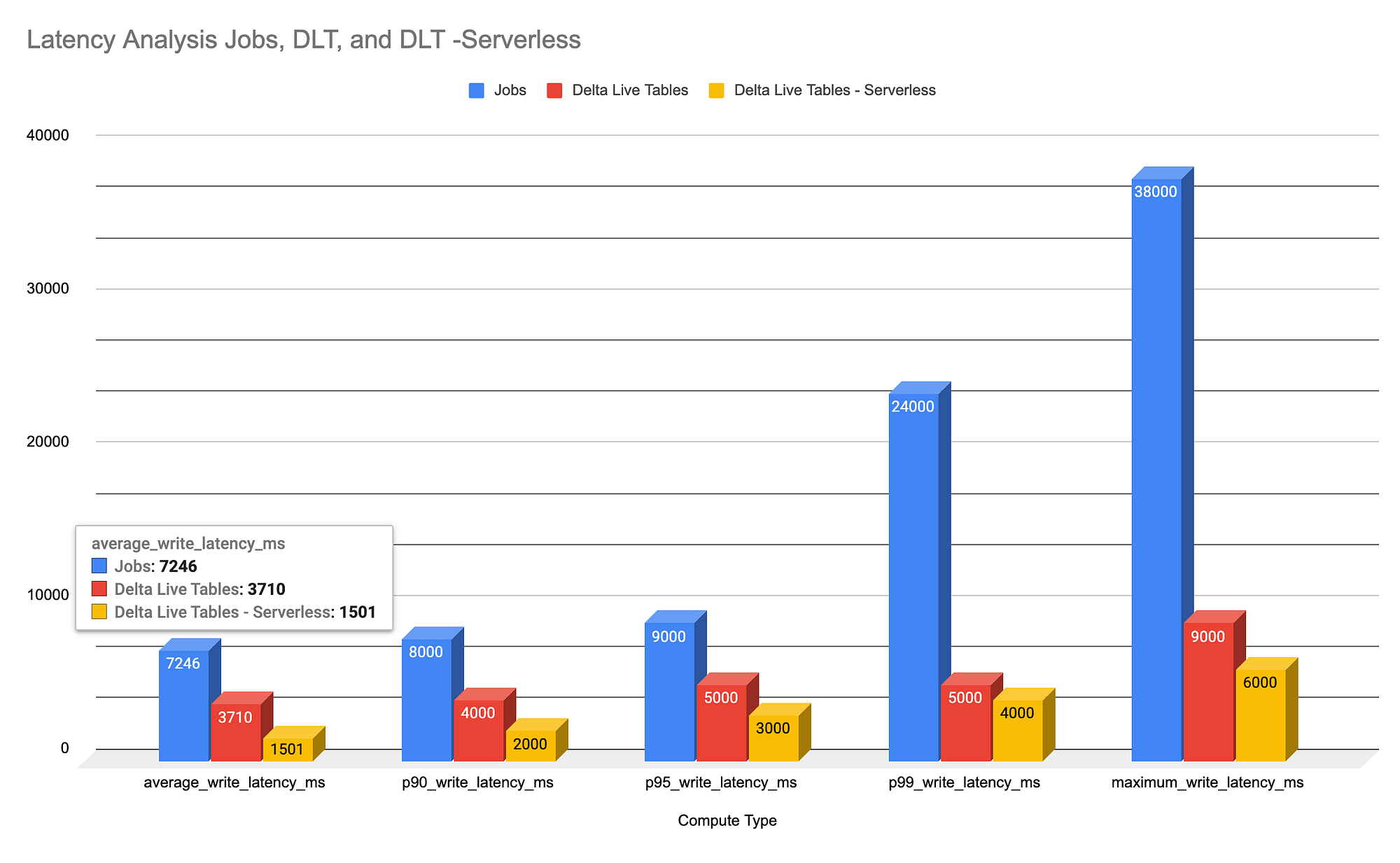
This blog post benchmarks three powerful options available on the Databricks platform for ingesting streaming data from Apache Kafka into Delta Lake: Databricks Jobs, Delta Live Tables (DLT), and Delta Live Tables Serverless (DLT Serverless). The primary objective is to evaluate and compare the end-to-end latency of these approaches when ingesting data from Kafka into Delta tables.
Latency is a crucial metric, as it directly impacts the freshness and timeliness of data available for downstream analytics and decision-making processes. It’s important to note that all three tools leverage Apache Spark’s Structured Streaming under the hood.
“Breaking the myth: Ingest from Kafka to Delta at scale in just 1.5 seconds with Delta Live Tables Serverless — up to 80% faster than traditional methods!”
Benchmark Setup
Criteria
The key metric measured was latency — the duration from when a row is produced in Kafka to when it becomes available in Delta Lake. Latency was meticulously measured over an extended period to ensure precision and account for variability.
Input Kafka Feed
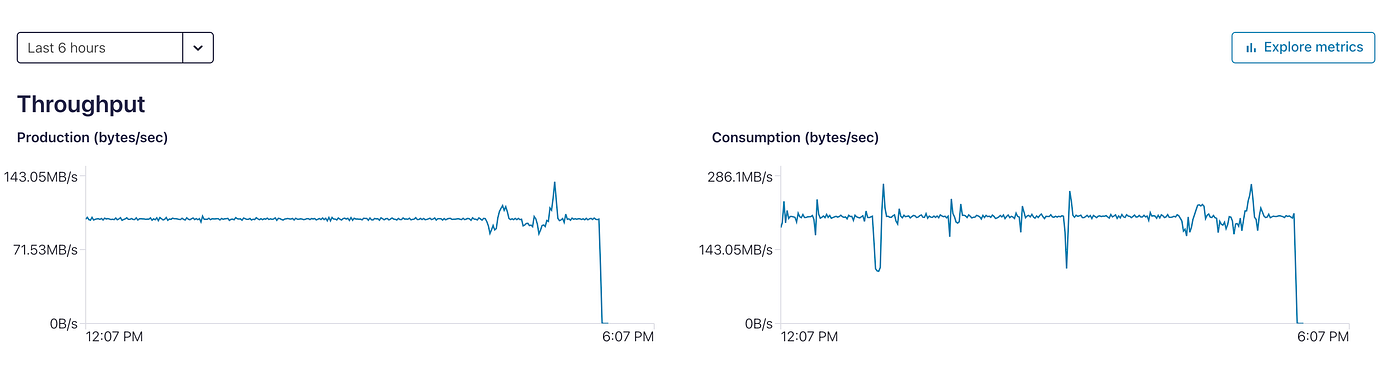
For our benchmarks, we utilized a Kafka feed churning out data at a rate of 100 rows per second, each approximately 1MB in size which is 100 MB/Second . Annually, this sums up to a staggering 3.15 petabytes, making it a rigorous testbed for evaluating the ingestion capabilities of our selected tools.
I used Confluent Cloud to setup Kafka cluster with 6 partitions and it took less than 5 minutes and they gave me 300$ of credits for experimentation.
Tools Compared
- Databricks Jobs: Utilizes Apache Spark Structured Streaming for reading from Kafka and writing to Delta Lake tables. It provides flexibility in job configuration and scheduling but requires manual management of cluster resources.
- Delta Live Tables (DLT): Employs a declarative approach for data ingestion from Kafka into Delta Lake, automatically managing infrastructure and simplifying pipeline development.
- Delta Live Tables Serverless (DLT Serverless): Leverages a serverless model to further simplify infrastructure management while performing the same ingestion tasks as DLT. It offers automatic scaling and resource optimization.
How was latency measured?
Latency is measured by calculating the time difference in milliseconds between the timestamps of consecutive streaming updates to a table. This is done by subtracting the timestamp of a previous update from the timestamp of the current update for each sequential commit, allowing an analysis of how long each update takes to process relative to the previous one. The analysis is currently limited to the last 300 commits, but this number can be adjusted as needed.
from pyspark.sql import DataFrame

def run_analysis_about_latency(table_name: str) -> DataFrame:
    # SQL command text formatted as a Python multiline string
    sql_code = f"""
        -- Define a virtual view of the table's history
        WITH VW_TABLE_HISTORY AS (
          -- Describe the historical changes of the table
          DESCRIBE HISTORY {table_name}
        ),

        -- Define a view to calculate the timestamp of the previous write operation
        VW_TABLE_HISTORY_WITH_previous_WRITE_TIMESTAMP AS (
          SELECT
            -- Calculate the timestamp of the last write operation before the current one
            lag(timestamp) OVER (
              PARTITION BY 1
              ORDER BY version
            ) AS previous_write_timestamp,
            timestamp,
            version
          FROM
            VW_TABLE_HISTORY
          WHERE
            operation = 'STREAMING UPDATE'
        ),

        -- Define a view to analyze the time difference between consecutive commits
        VW_BOUND_ANALYSIS_TO_N_COMMITS AS (
          SELECT
            -- Calculate the time difference in milliseconds between the previous and current write timestamps
            TIMESTAMPDIFF(
              MILLISECOND,
              previous_write_timestamp,
              timestamp
            ) AS elapsed_time_ms
          FROM
            VW_TABLE_HISTORY_WITH_previous_WRITE_TIMESTAMP
          ORDER BY
            version DESC
          LIMIT
            300  -- Analyze only the last 300 commits
        )

        -- Calculate various statistics about the write latency
        SELECT
          avg(elapsed_time_ms) AS average_write_latency,
          percentile_approx(elapsed_time_ms, 0.9) AS p90_write_latency,
          percentile_approx(elapsed_time_ms, 0.95) AS p95_write_latency,
          percentile_approx(elapsed_time_ms, 0.99) AS p99_write_latency,
          max(elapsed_time_ms) AS maximum_write_latency
        FROM
          VW_BOUND_ANALYSIS_TO_N_COMMITS
    """
    # Execute the SQL query using Spark's SQL module
    display(spark.sql(sql_code))
Data Ingestion
This code sets up a streaming data pipeline using Apache Spark to efficiently ingest data from a Kafka topic. It defines a schema tailored to the expected data types and columns in the Kafka messages, including vehicle details, geographic coordinates, and text fields.The read_kafka_stream function initializes the streaming process, configuring secure and reliable connections to Kafka, subscribing to the specified topic, and handling data across multiple partitions for improved processing speed. The stream decodes JSON-formatted messages according to the defined schema and extracts essential metadata.
from pyspark.sql.types import StructType, StringType, FloatType
from pyspark.sql.functions import *
# Define the schema based on the DataFrame structure you are writing to Kafka
schema = StructType() \
    .add("event_id", StringType()) \
    .add("vehicle_year_make_model", StringType()) \
    .add("vehicle_year_make_model_cat", StringType()) \
    .add("vehicle_make_model", StringType()) \
    .add("vehicle_make", StringType()) \
    .add("vehicle_model", StringType()) \
    .add("vehicle_year", StringType()) \
    .add("vehicle_category", StringType()) \
    .add("vehicle_object", StringType()) \
    .add("latitude", StringType()) \
    .add("longitude", StringType()) \
    .add("location_on_land", StringType()) \
    .add("local_latlng", StringType()) \
    .add("zipcode", StringType()) \
    .add("large_text_col_1", StringType()) \
    .add("large_text_col_2", StringType()) \
    .add("large_text_col_3", StringType()) \
    .add("large_text_col_4", StringType()) \
    .add("large_text_col_5", StringType()) \
    .add("large_text_col_6", StringType()) \
    .add("large_text_col_7", StringType()) \
    .add("large_text_col_8", StringType()) \
    .add("large_text_col_9", StringType())

def read_kafka_stream():
    kafka_stream = (spark.readStream
      .format("kafka")
      .option("kafka.bootstrap.servers", kafka_bootstrap_servers_tls )
      .option("subscribe", topic )
      .option("failOnDataLoss","false")
      .option("kafka.security.protocol", "SASL_SSL")
      .option("kafka.sasl.mechanism", "PLAIN")
      .option("kafka.sasl.jaas.config", f'kafkashaded.org.apache.kafka.common.security.plain.PlainLoginModule required username="{kafka_api_key}" password="{kafka_api_secret}";')
      .option("minPartitions",12)
      .load()
      .select(from_json(col("value").cast("string"), schema).alias("data"), "topic", "partition", "offset", "timestamp", "timestampType" )
      .select("topic", "partition", "offset", "timestamp", "timestampType", "data.*")
    )
    return kafka_stream
Explanation:
- Connection Setup: Connects to Kafka using specific bootstrap servers and includes security settings like SASL_SSL for encrypted and authenticated data transfer.
- Topic Subscription: Subscribes to a specified Kafka topic to continuously receive new data.
- Stream Configuration: Robustly configured to handle potential data loss and manage data across multiple partitions to boost processing speed.
- Data Transformation: Uses
from_jsonto decode JSON messages according to the established schema, transforming them into a structured format within Spark. - Metadata Extraction: Extracts essential metadata like the Kafka topic, partition, and message timestamps.
This setup optimizes data ingestion from Kafka into Spark and prepares the data for further processing or integration into storage systems like Delta Lake.
Additional code for Databricks Jobs
Configuration: This method involves setting up a Databricks job and cluster resources, although it allows for flexible scheduling and monitoring of ingestion processes it but requires understanding of choosing the right compute.
(
  read_kafka_stream()
  .writeStream
  .option("checkpointLocation",checkpoint_location_for_delta)
  .trigger(processingTime='1 second')
  .toTable(target)
)
Additional code for Delta Live Tables
Configuration: Delta Live Tables manage infrastructure automatically, providing a simpler, declarative approach to building data pipelines.
This code snippet uses the Delta Live Tables (DLT) API to define a data table that ingests streaming data from Kafka. The @dlt.table decorator specifies the table’s name (to be replaced with your desired table name) and sets the pipeline to poll Kafka every second. This rapid polling supports near-real-time data processing needs. The function dlt_kafka_stream() calls read_kafka_stream(), integrating Kafka streaming directly into DLT for streamlined management and operation within the Databricks environmen
@dlt.table(name="REPLACE_DLT_TABLE_NAME_HERE",
           spark_conf={"pipelines.trigger.interval" : "1 seconds"})
def dlt_kafka_stream():
    read_kafka_stream()
Conclusion
Our benchmarks show that Delta Live Tables Serverless stands out in latency performance and operational simplicity, making it highly suitable for scenarios with varying data loads. Meanwhile, Databricks Jobs and Delta Live Tables also offer viable solutions.
- Latency Comparison: The serverless version of Delta Live Tables outperforms the others in terms of latency across all measured percentiles.
- Operational Complexity: Delta Live Tables Serverless offers the least complex setup, with no need for manual infrastructure management, followed by Delta Live Tables and then Databricks Jobs.
Why Delta Live Tables Serverless Outperforms Standard Delta Live Tables
A key factor contributing to the superior performance of Delta Live Tables Serverless over its non-serverless counterpart is its use of Stream Pipelining. Unlike standard Structured Streaming, which processes microbatches sequentially, DLT Serverless handles them concurrently. This not only enhances throughput but significantly improves latency and overall compute resource utilization. Stream Pipelining is a default feature in serverless DLT pipelines, further optimizing performance for streaming data workloads like data ingestion.
Additionally, Vertical Autoscaling plays a pivotal role in enhancing the efficiency of DLT Serverless. This feature complements the horizontal autoscaling capabilities of Databricks Enhanced Autoscaling by automatically choosing the most cost-effective instance types needed to run the DLT pipelines without risking out-of-memory failures. It adeptly scales up to larger instances when more resources are required and scales down when memory utilization is consistently low. This dynamic adjustment ensures that both driver and worker nodes are optimally scaled based on real-time demands. Whether updating pipelines in production mode or manually in development, vertical autoscaling swiftly allocates larger instances following out-of-memory errors, thereby maintaining uninterrupted service and optimizing resource allocation.
Together, Stream Pipelining and Vertical Autoscaling not only reduce operational complexities but also enhance the reliability and cost-efficiency of Serverless DLT pipelines. These features make Serverless DLT an ideal choice for managing fluctuating data ingestion loads with minimal manual intervention, leading to faster, more efficient data pipeline executions.
Footnote:
Thank you for taking the time to read this article. If you found it helpful or enjoyable, please consider clapping to show appreciation and help others discover it. Don’t forget to follow me for more insightful content, and visit my website CanadianDataGuy.com for additional resources and information. Your support and feedback are essential to me, and I appreciate your engagement with my work.