Author name: CanadianDataGuy

Blog, Stream, Streaming Aggregation

SPARK STREAM AGGREGATION: A BEGINNER’S JOURNEY WITH PRACTICAL CODE EXAMPLE

Welcome to the fascinating world of Spark Stream Aggregation! This blog is tailored for beginners, featuring hands-on code examples from a real-world scenario of processing vehicle data. I suggest reading the blog first without the code and then reading the code with the blog. Setting up Spark Configuration, Imports & Parameters First, let’s understand our setup. We configure the Spark environment to use RocksDB for state management, enhancing the efficiency of our stream processing: spark.conf.set(“spark.sql.streaming.stateStore.providerClass”, “com.databricks.sql.streaming.state.RocksDBStateStoreProvider”) !pip install faker_vehicle !pip install faker from faker import Faker from faker_vehicle import VehicleProvider from pyspark.sql import functions as F from pyspark.sql.types import StringType import uuid from pyspark.sql.streaming import StreamingQuery import logging logging.basicConfig(level=logging.INFO, format=’%(asctime)s – %(name)s – %(levelname)s – %(message)s’) logger = logging.getLogger(__name__) # define schema name and where should the table be stored schema_name = “test_streaming_joins” schema_storage_location = “/tmp/CHOOSE_A_PERMANENT_LOCATION/” target_table = f”{schema_name}.streaming_aggregation” checkpoint_location= f”{schema_storage_location}{target_table}/_checkpoint/”, silver_target_table= f”{schema_name}.silver_streaming” silver_checkpoint_locattion = f”{schema_storage_location}{silver_target_table}/_checkpoint/”, column_to_watermark_on = “timestamp” how_late_can_the_data_be = “3 minutes” create_schema_sql = f””” CREATE SCHEMA IF NOT EXISTS {schema_name} COMMENT ‘This is {schema_name} schema’ LOCATION ‘{schema_storage_location}’; “”” logger.info(f”Executing SQL: {create_schema_sql}”) spark.sql(create_schema_sql) Simulating Data Streams Using the Faker library, we simulate a vehicle data stream. This approach helps us create a realistic data processing environment that is crucial for our learning: # Using Faker to define functions for fake data generation fake = Faker() fake.add_provider(VehicleProvider) event_id = F.udf(lambda: str(uuid.uuid4()), StringType()) vehicle_year_make_model = F.udf(fake.vehicle_year_make_model) vehicle_year_make_model_cat = F.udf(fake.vehicle_year_make_model_cat) vehicle_make_model = F.udf(fake.vehicle_make_model) vehicle_make = F.udf(fake.vehicle_make) vehicle_model = F.udf(fake.vehicle_model) vehicle_year = F.udf(fake.vehicle_year) vehicle_category = F.udf(fake.vehicle_category) vehicle_object = F.udf(fake.vehicle_object) latitude = F.udf(fake.latitude) longitude = F.udf(fake.longitude) location_on_land = F.udf(fake.location_on_land) local_latlng = F.udf(fake.local_latlng) zipcode = F.udf(fake.zipcode) # COMMAND ———- # MAGIC %md # MAGIC ### Generate Streaming source data at your desired rate # COMMAND ———- # Generate streaming data def generated_vehicle_and_geo_df(rowsPerSecond: int =100, numPartitions: int = 10): logger.info(“Generating vehicle and geo data frame…”) return ( spark.readStream.format(“rate”) .option(“numPartitions”, numPartitions) .option(“rowsPerSecond”, rowsPerSecond) .load() .withColumn(“event_id”, event_id()) .withColumn(“vehicle_year_make_model”, vehicle_year_make_model()) .withColumn(“vehicle_year_make_model_cat”, vehicle_year_make_model_cat()) .withColumn(“vehicle_make_model”, vehicle_make_model()) .withColumn(“vehicle_make”, vehicle_make()) .withColumn(“vehicle_year”, vehicle_year()) .withColumn(“vehicle_category”, vehicle_category()) .withColumn(“vehicle_object”, vehicle_object()) .withColumn(“latitude”, latitude()) .withColumn(“longitude”, longitude()) .withColumn(“location_on_land”, location_on_land()) .withColumn(“local_latlng”, local_latlng()) .withColumn(“zipcode”, zipcode()) ) # You can uncomment the below display command to check if the code in this cell works display(generated_vehicle_and_geo_df()) Aggregation Modes in Spark Streaming Stream Aggregation in Spark lets us process continuous data streams. Our code demonstrates how to generate and aggregate streaming data. Spark Streaming provides three primary modes for data output during stream processing: Complete Mode Update Mode Each mode caters to different requirements, offering flexibility in streaming applications. Applying Aggregation in Practice Our code showcases these modes in action, applying them to our simulated vehicle data stream: def streaming_aggregation(rows_per_second: int = 100, num_partitions: int = 10, how_late_can_the_data_be :str = “30 minutes”, window_duration: str = “1 minutes”, checkpoint_location: str = checkpoint_location, output_table_name: str = target_table) -> StreamingQuery: “”” Aggregate streaming data and write to a Delta table. Parameters: – rows_per_second (int): Number of rows per second for generated data. – num_partitions (int): Number of partitions for the generated data. – window_duration (str): Window duration for aggregation. – checkpoint_location (str): Path for checkpointing. – output_table_name (str): Name of the output Delta table. Returns: – StreamingQuery: Spark StreamingQuery object. “”” logger.info(“Starting streaming aggregation…”) raw_stream = generated_vehicle_and_geo_df(rows_per_second, num_partitions) aggregated_data = ( raw_stream .withWatermark(column_to_watermark_on, how_late_can_the_data_be) .groupBy( F.window(column_to_watermark_on, window_duration), “zipcode” ) .agg( F.min(“vehicle_year”).alias(“oldest_vehicle_year”) ) ) query = ( aggregated_data .writeStream .queryName(f”write_stream_to_delta_table: {output_table_name}”) .format(“delta”) .option(“checkpointLocation”, checkpoint_location) .outputMode(“append”) .toTable(output_table_name) # This actually starts the streaming job ) logger.info(f”Streaming query started with ID: {query.id}”) logger.info(f”Current status of the query: {query.status}”) logger.info(f”Recent progress updates: {query.recentProgress}”) # If you want to programmatically stop the query after some condition or time, you can do so. # For the sake of this example, I am NOT stopping it. But if you need to, you can invoke: # query.stop() # logger.info(“Streaming query stopped.”) return query streaming_aggregation( checkpoint_location = checkpoint_location, output_table_name = target_table, how_late_can_the_data_be = “5 minutes” ) What is most critical to understand is the Watermarking column. Best Practices and Considerations Download the code https://github.com/jiteshsoni/material_for_public_consumption/blob/main/notebooks/spark_stream_aggregations.py Conclusion This blog provides a beginner-friendly introduction to Spark Stream Aggregation, supported by practical code examples. Dive in and explore the world of real-time data processing with Spark! Thank You for Reading! I hope you found this article helpful and informative. If you enjoyed this post, please consider giving it a clap 👏 and sharing it with your network. Your support is greatly appreciated! — **CanadianDataGuy**

Blog, Delta

SOLVING DELTA TABLE CONCURRENCY ISSUES

Delta Lake is a powerful technology for bringing ACID transactions to your data lakes. It allows multiple operations to be performed on a dataset concurrently. However, dealing with concurrent operations can sometimes be tricky and may lead to issues such as ConcurrentAppendException, ConcurrentDeleteReadException, and ConcurrentDeleteDeleteException. In this blog post, we will explore why these issues occur and how to handle them effectively using a Python function, and how to avoid them with table design and using isolation levels and write conflicts. Why Do These Issues Happen? Understanding Isolation Levels: Serializable vs. WriteSerializable Isolation levels in a database control how much transactions are protected from each other’s changes. Delta Lake on Databricks offers two such levels: Serializable and WriteSerializable. 1. Serializable: — This is the highest level of isolation. — It ensures that all write and read operations are done in a specific order, just like how they appear in the table’s history. — This means operations are carried out one by one, maintaining the order and ensuring the final result is as expected. 2. WriteSerializable (Default): — This level is a bit more relaxed compared to Serializable. — It guarantees order only for write operations, not for reads. — Even though it’s more relaxed, it’s still more strict than the Snapshot isolation level. — This level is used by default as it offers a good mix of data consistency and availability for most operations. Solution 1: Setting the Isolation Level: Solution 2: Avoiding Conflicts Using Partitioning and Disjoint Command Conditions When working with tables, sometimes two operations can clash or conflict, especially if they are working on the same set of files. This can cause problems and errors. But, there’s a way to avoid this! You can organize or partition your table based on certain columns that are often used in operations. This way, different operations work on different parts of the table, preventing them from clashing. For example, imagine two commands — one is updating the table for dates after January 1, 2010, and another is deleting from the table for dates before January 1, 2010. These two can clash if the table is not organized by date, as both might try to change the same files. But if you partition the table by date, these operations won’t conflict, making things smooth and error-free. However, be careful while choosing the column for partitioning. If you choose a column that has a lot of unique values, it can create a large number of subdirectories. This can lead to other issues, affecting the performance of operations on the table. By using these strategies and understanding the insights from Databricks regarding isolation levels, row-level concurrency, and write conflicts, you can make your Delta operations more robust, reliable, and efficient. Solution 3: Code block with exponential retry The Python code below offers a robust solution to address this challenge. It is designed to manage concurrent write operations to a Delta table or path by intelligently retrying the operation in the event of specific concurrent exceptions. Streaming_write_with_concurrent_retry takes parameters such as the data stream, maximum attempts, and others to provide flexibility and control. It employs a while loop to attempt the write operation continuously and waits for its completion. In case of concurrent exceptions, it increments the attempt counter and calculates the sleep time using an exponential backoff strategy before retrying the operation. This approach ensures that the write operation is eventually successful, providing reliability and efficiency in handling concurrent operations on Delta tables. Explore the code below to understand its workings and integrate it into your projects to enhance concurrent operations handling. from datetime import datetime from time import sleep from delta.exceptions import ( ConcurrentAppendException, ConcurrentDeleteReadException, ConcurrentDeleteDeleteException, ) import math def streaming_write_with_concurrent_retry( stream, max_attempts=3, indefinite=False, table=None, path=None ): “”” Handles concurrent write operations to a Delta table or path by retrying the operation in case of specific concurrent exceptions. :param stream: The data stream to be written. :param max_attempts: The maximum number of retry attempts. Default is 3. :param indefinite: If True, will keep retrying indefinitely. Default is False. :param table: The Delta table to write to. :param path: The path to write to. :return: The result of writer.awaitTermination(). “”” attempt = 0 # Initialize attempt counter while True: try: # Choose the writer based on whether table or path is provided if table: writer = stream.table(table) elif path: writer = stream.start(path) else: writer = stream.start() # Attempt to write and wait for termination return writer.awaitTermination() # Handle concurrent exceptions except ( ConcurrentAppendException, ConcurrentDeleteReadException, ConcurrentDeleteDeleteException, ) as e: # Increment attempt counter attempt += 1 # If indefinite is False and attempts have reached max_attempts, raise the exception if not indefinite and attempt >= max_attempts: raise e from None # Calculate sleep time using exponential backoff strategy sleep_time = min(120, math.pow(2, attempt)) # Sleep for the calculated time before retrying sleep(sleep_time) Solution 4: Row-Level Concurrency (Advanced Feature)? Available only on Delta tables with deletion vectors enabled and on Photon-enabled compute running Databricks Runtime 14.0 and above. Reference Isolation levels and write conflicts on Databricks *Learn about the isolation levels and potential conflicts when performing concurrent transactions on tables on…*docs.databricks.com Thank You for Reading! I hope you found this article helpful and informative. If you enjoyed this post, please consider giving it a clap 👏 and sharing it with your network. Your support is greatly appreciated! — **CanadianDataGuy**

Best Practices, Blog

Databricks SQL Dashboards Guide: Tips and Tricks to Master Them

Welcome to the world of Databricks SQL Dashboards! You’re in the right place if you want to learn how to go beyond just building visualizations and add some tricks to your arsenal. This guide will walk you through creating, managing, and optimizing your Databricks SQL dashboards. 1. Getting Started with Viewing and Organizing Dashboards: 2. Tags are your friend 3. Cloning: Replicating Success: 4. Harnessing the Power of Query Parameters: 5. Editing and Customizing Your Dashboard: 6. Keeping Your Data Fresh with Refreshes: 7. Stay Updated with Dashboard Subscriptions: 8. Managing and Optimizing Dashboards: In conclusion, Databricks SQL dashboards offer a versatile data visualization and analysis platform. With this step-by-step guide, you’re well on your way to mastering the art of creating, managing, and optimizing your dashboards. Dive in and explore the world of data with Databricks!

Best Practices, Blog

Optimizing Databricks SQL: Achieving Blazing-Fast Query Speeds at Scale

In this data age, delivering a seamless user experience is paramount. While there are numerous ways to measure this experience, one metric stands tall when evaluating the responsiveness of applications and databases: the P99 latency. Especially vital for SQL queries, this seemingly esoteric number is, in reality, a powerful gauge of the experience we provide to our customers. Why is it so crucial? And how can we optimize it to ensure our databases aren’t just fast, but consistently reliable for 99% of our users? Join us as we demystify P99 latency and delve into strategies to fine-tune it in Databricks SQL. What is P99 Latency? The P99 latency (also known as the 99th percentile latency) for SQL queries is a metric used to measure the response time of SQL queries in a database system. It represents the latency at which 99% of the queries have a response time less than or equal to the P99 latency value, and 1% have a response time greater than the P99 latency value. In other words, P99 latency helps you understand the worst-case response time for most of your SQL queries. It is often used to evaluate the performance of a database system and ensure that the vast majority of queries are responding quickly, even under heavy load. For example, if the P99 latency for a particular SQL query is 100 milliseconds, it means that 99% of the time, that query will execute in 100 milliseconds or less. However, in 1% of cases, it may take longer than 100 milliseconds. To achieve a P99 latency of 5 seconds in Databricks SQL, you can follow these steps: If you need to power an application with minimum latency, it’s possible to pre-cache data using specific commands. However, it’s important to take caution while using these commands as misconfiguration can cause more harm than good. It’s recommended to reach out to me or your Databricks representative for the command and have the scenario validated with Databricks before implementing it. I have not included the command in the blog to avoid any mishaps. Reference: 3. https://www.youtube.com/watch?v=rJDkfRPUebw&t=629s 

Blog, forEachBatch, Spark, Stream

Simplifying Real-time Data Processing with Spark Streaming’s foreachBatch with working code

Comprehensive guide to implementing a fully operational Streaming Pipeline that can be tailored to your specific needs. In this working example, you will learn how to parameterize the ForEachBatch function. Spark Streaming & foreachBatch Spark Streaming is a powerful tool for processing streaming data. It allows you to process data as it arrives, without having to wait for the entire dataset to be available. This can be very useful for applications that need to respond to changes in data in real time. One of the features of Spark Streaming is the foreachBatch() method. This method allows you to apply a custom function to each batch of data as it arrives. This can be useful for a variety of tasks, such as: The foreachBatch() method is a powerful tool that can be used to extend the capabilities of Spark Streaming. In this blog post, we will take a closer look at how to use foreachBatch(). Introducing foreachBatch: foreachBatch is a method provided by Spark Streaming that allows developers to apply arbitrary operations on the output of a streaming query. It acts as a bridge between the streaming world and the structured world of DataFrames and Datasets. This means that we can leverage the rich functionality of Spark’s structured APIs to process real-time data efficiently. The Power of foreachBatch: The foreachBatch operation enables developers to perform batch-like operations on streaming data. Instead of processing each individual record, which can be inefficient, foreachBatch processes the data in micro-batches, offering better performance and resource utilization. This approach also provides the flexibility to leverage the full power of Spark’s DataFrames, including various transformations and aggregations, to perform complex computations on streaming data. Implementing foreachBatch: To use foreachBatch, you need to define a function that takes two arguments: the batch identifier and the DataFrame representing the micro-batch of data. Inside this function, you can apply any transformations or computations required on the streaming data. You can use Spark’s SQL, DataFrame, or Dataset APIs to manipulate the data and write the results to any external systems, such as databases or file systems. Benefits of foreachBatch: Code & Setup Here’s how we can use foreachBatch to achieve this: ∘ Define parameters for the job ∘ Create a Streaming source ∘ Define custom processing logic and parameters ∘ Create an instance of forEachBatchProcessor Class with the parameters ∘ Orchestrate the job ∘ Look at the output table ∘ Clean Up Define parameters for the job target_table_name = “for_each_batch_paramerterize” check_point_location = f”/tmp/delta/{target_table_name}/_checkpoints/” dedupe_colum_name =”hash” Create a Streaming source We will create a synthetic dataset. generated_df = ( spark.readStream .format(“rate”) .option(“numPartitions”, 4) .option(“rowsPerSecond”, 1 * 1000) .load() .selectExpr( “md5( CAST (value AS STRING) ) as md5″ ,”value” ,”value%1000000 as hash” ) ) Define custom processing logic and parameters class forEachBatchProcessor: def __init__(self, dedupe_column: str, filter_criteria:str, passed_value: int): self.dedupe_column = dedupe_column self.filter_criteria = filter_criteria self.passed_value = passed_value def print_attributes(self): attributes = vars(self) print( “\n”.join([f”{attr}: {value}” for attr, value in attributes.items()]) ) def make_changes_using_the_micro_batch(self, microBatchOutputDF, batchId: int): self.print_attributes() print(f”Processing batchId: {batchId}”) # Your processing logic using the parameter view_name = f”updates_for_batchId_{batchId}” microBatchOutputDF.createOrReplaceTempView(view_name) sql_logic = f””” SELECT * ,{self.passed_value} as passed_value ,{batchId} as batch_id FROM ( SELECT * ,rank() over(partition by {self.dedupe_column} order by value desc) as dedupe FROM {view_name} WHERE {self.filter_criteria} ) WHERE dedupe =1 “”” print(f”Processing sql_logic: {sql_logic}”) to_be_written_df = microBatchOutputDF.sparkSession.sql(sql_logic).drop(“dedupe”) to_be_written_df.write.mode(“append”).saveAsTable(target_table_name) Create an instance of forEachBatchProcessor Class with the parameters instantiateForEachBatchProcessor = forEachBatchProcessor( dedupe_column = dedupe_colum_name, filter_criteria = “1=1”, passed_value = 3 ) Orchestrate the job ( generated_df .writeStream #.trigger(availableNow=True) .trigger(processingTime=’10 seconds’) .option(“checkpointLocation”, check_point_location) .option(“queryName”, “ParameterizeForEachBatch”) .foreachBatch(instantiateForEachBatchProcessor.make_changes_using_the_micro_batch) .start() ) Look at the output table display(spark.read.table(target_table_name)) Clean Up spark.sql(f””” DROP TABLE IF EXISTS {target_table_name} “””) dbutils.fs.rm(check_point_location,True) Conclusion: Apache Spark Streaming’s foreachBatch operation is a powerful tool for simplifying real-time data processing. By bridging the gap between the streaming and structured worlds, it enables developers to perform batch-like operations on streaming data efficiently. Leveraging the rich functionality of Spark’s DataFrames, foreachBatch empowers users to process and analyze real-time data with ease. Whether you’re performing aggregations, transformations, or writing data to external systems, foreachBatch offers a flexible and scalable solution for real-time streaming applications. Footnote: Thank you for taking the time to read this article. If you found it helpful or enjoyable, please consider clapping to show appreciation and help others discover it. Don’t forget to follow me for more insightful content, and visit my website **CanadianDataGuy.com** for additional resources and information. Your support and feedback are essential to me, and I appreciate your engagement with my work. Download the code I want to emphasize that my blog posts are designed to be practical resources that you can readily use in your own environments. By providing code examples with careful attention to best practices, I aim to simplify the implementation of real-time data processing solutions. I encourage you to explore the blog, copy the code snippets, and adapt them to your specific needs. With these resources, you’ll be equipped to accelerate your development process and unlock the power of Spark Streaming. Dive in, leverage the code, and start building your real-time data processing pipelines with confidence! Go Build! Canadian Data Guy!

Blog, Delta

Delta vs. Parquet: A Deep Dive into Big Data Storage Solutions

Unlocking the intricacies of big data storage solutions is pivotal in today’s data-driven landscape. As organizations grapple with vast amounts of data, choosing between storage formats like Delta and Parquet becomes crucial. Diving deep into their technical nuances, this article highlights why Delta is emerging as the preferred choice for many. From ACID transactions to schema evolution, discover the game-changing features that set Delta apart in the competitive world of data storage. 1. Introduction to Delta and Parquet Parquet: An open-source columnar storage format developed under the Apache Software Foundation. It is designed to be compatible with a wide variety of data processing tools in the Hadoop ecosystem. Delta: Delta Lake is more than just a file format; it’s a storage layer that brings ACID transactions to big data workloads on top of Spark. 2. Technical Differences a. ACID Transactions: b. Schema Evolution: c. Time Travel: d. Storage Efficiency: e. Merge, Update, and Delete: 3. Performance Insights 4. Compatibility and Ecosystem 5. The Verdict While Parquet is a robust columnar storage format that has served the big data community well, Delta brings in features that cater to the evolving needs of data engineering and data science teams. Its emphasis on transactional integrity, combined with advanced optimizations, positions Delta as a formidable player in the big data storage arena.

Best Practices, Blog

How to Cut Your Data Processing Costs by 30% with Graviton

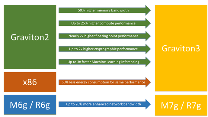
What is AWS Graviton ? AWS Graviton is a family of Arm-based processors that are designed by AWS to provide cost-effective and high-performance computing for cloud workloads. Graviton processors are built using 64-bit Arm, which are optimized for power efficiency and performance. They offer a more cost-effective alternative to traditional x86-based processors, making them a popular choice for running a variety of workloads on AWS. With Graviton, you can enjoy lightning-fast data processing speeds while saving money on your infrastructure costs. Plus, Graviton is compatible with all your favorite tools and applications, so you can seamlessly integrate it into your existing workflow. Overall, AWS Graviton offers a flexible and cost-effective alternative to traditional x86-based processors, making it a popular choice for customers who are looking to optimize their cloud computing costs without sacrificing performance or reliability. Cost Savings If you look at the screenshot below, you will find Graviton cheaper than every other series. **Decipher instance name: c6g.xlarge: **C stands for compute series, 6 stands for a series number, g stands for Graviton, and xLarge means 4 vCPU. Compute Intensive (C Series) c6g.xlarge is 12.5% cheaper than the next cheapest instance. General Purpose (M Series) m6g.xlarge is ~12.2% cheaper than the next cheapest instance. Memory Intensive ( R Series) r6g.xlarge is ~12.5% cheaper than the next cheapest instance. This is complicated. Help me choose ? Let me break down the AWS instance series into simple parts. Think about how much memory you get per core, and the price increases as the memory increases. I recommend that customers start with general purpose, get a baseline runtime, and then try different series. The best way to gauge what instance family would work is to identify or categorize if the workload is compute-bound, memory-bound or network bound. Launch of new Graviton 3 series in 2023 Here are some benefits of the new Graviton 3 series; the price is ~10% more expensive Graviton 2. However, it’s still cheaper than the M6 a instance. M6g ($ 0.154) < M7g ($ 0.1632) < M6a ( $0.1728 ) New Graviton3-Based General Purpose (m7g) and Memory-Optimized (r7g) Amazon EC2 Instances | Amazon… *We’ve come a long way since the launch of the m1.small instance in 2006, adding instances with additional memory…*aws.amazon.com Conclusion As you can see, the price saving is at least ~12%, and AWS claims 40% better price performance due to faster processors. Thus, in reality, you should be able to save 12–40% cost savings at least. In my real-world experience, I have seen 20–30% cost savings. Footnote: Thank you for taking the time to read this article. If you found it helpful or enjoyable, please consider clapping to show appreciation and help others discover it. Don’t forget to follow me for more insightful content, and visit my website **CanadianDataGuy.com** for additional resources and information. Your support and feedback are essential to me, and I appreciate your engagement with my work.

Blog

A Productive Life: How to Parallelize Code Execution in Python

Asynchronous programming has become increasingly popular in recent years, especially in web development, where it is used to build high-performance, scalable applications. Python has built-in support for asynchronous programming through the asyncio module, which provides a powerful framework for writing asynchronous code. In this blog post, we will explore the asyncio module in Python 3.10 and learn how to run tasks in parallel using the new features introduced in this version. We will explore 3 examples here: Example 1: Asyncio Tasks / create_task() In asyncio, a task is a unit of work that is scheduled to run on the event loop. Tasks are created from coroutines, which are functions that are defined using the async def syntax and that can suspend their execution using the await keyword. To create a task, we use the asyncio.create_task() function, which takes a coroutine as its argument and returns a Task object. We can then schedule the task to run on the event loop using the await keyword. Here’s an example: import asyncio async def function_which_will_run_in_parallel(): # Add what you want to do here print(‘function_which_will_run_in_parallel completed’) # Orchestrate function async def main(): task = asyncio.create_task(function_which_will_run_in_parallel()) await task asyncio.run(main()) In this example, we define a simple function_which_will_run_in_parallel() that waits for one second and then prints a message. In the main() function, we create a Task object using asyncio.create_task() and pass it the function. We then await the completion of the task using await task. When we run the main() using asyncio.run(), the Task object is created and scheduled on the event loop, which runs the function_which_will_run_in_parallel() function asynchronously. Once the function_which_will_run_in_parallel() function is complete, the Task object is marked as done, and the program exits. Example 2: Running Tasks in Parallel In asyncio, we can run tasks in parallel using the asyncio.gather() function. This function takes one or more coroutines/functions as its arguments and returns a list of their results. Here’s an example: import asyncio async def coroutine1(): await asyncio.sleep(1) return ‘Coroutine 1 completed’ async def coroutine2(): await asyncio.sleep(2) return ‘Coroutine 2 completed’ async def main(): results = await asyncio.gather(coroutine1(), coroutine2()) print(results) asyncio.run(main()) In this example, we define two coroutines, coroutine1() and coroutine2(), that wait for one and two seconds, respectively, before returning a message. In the main() coroutine function, we use the asyncio.gather() function to run the two coroutines in parallel. We pass coroutine1() and coroutine2() as its arguments and use await to wait for both coroutines to complete. When both coroutines are complete, the asyncio.gather() function returns a list of their results, which we print to the console. Example 3: Running tasks in parallel with a loop In this example, we define an asynchronous coroutine function fetch() that uses the aiohttp library to download the contents of a given URL. We then define the main() coroutine function that creates a list of URLs to download and uses asyncio.create_task() to create a task for each URL. We then use asyncio.gather() to wait for all tasks to complete and return their results. The async with aiohttp.ClientSession() context manager is used to create a session object that can be reused across multiple requests, which can improve performance. When we run the main() coroutine using asyncio.run(), it concurrently downloads the web pages from the list of URLs, and prints the number of bytes downloaded from each URL. This is just a simple example, but it demonstrates how asyncio can be used to concurrently perform I/O-bound tasks such as web page downloads. import asyncio import aiohttp async def fetch(session, url): async with session.get(url) as response: return await response.text() async def main(): urls = [ ‘https://example.com’, ‘https://google.com’, ‘https://facebook.com’, ‘https://twitter.com’, ‘https://linkedin.com’, ] async with aiohttp.ClientSession() as session: tasks = [asyncio.create_task(fetch(session, url)) for url in urls] results = await asyncio.gather(*tasks) for url, result in zip(urls, results): print(f”Downloaded {len(result)} bytes from {url}”) asyncio.run(main()) Conclusion Asyncio is a powerful framework for writing asynchronous code in Python, and with the new features introduced in Python 3.10, it has become even easier to run tasks in parallel. In this blog post, we learned how to create tasks using asyncio.create_task() and how to run tasks in parallel using `asyncio.gather() Footnote: Thank you for taking the time to read this article. If you found it helpful or enjoyable, please consider clapping to show appreciation and help others discover it. Don’t forget to follow me for more insightful content, and visit my website **CanadianDataGuy.com** for additional resources and information. Your support and feedback are essential to me, and I appreciate your engagement with my work.

Databricks, Delta, Spark, Stream, Stream-Stream

How to write your first Spark application with Stream-Stream Joins with working code.

Have you been waiting to try Streaming but cannot take the plunge? In a single blog, we will teach you whatever needs to be understood about Streaming Joins. We will give you a working code which you can use for your next Streaming Pipeline. The steps involved: Create a fake dataset at scaleSet a baseline using traditional SQLDefine Temporary Streaming ViewsInner Joins with optional WatermarkingLeft Joins with WatermarkingThe cold start edge case: withEventTimeOrderCleanup What is Stream-Stream Join? Stream-stream join is a widely used operation in stream processing where two or more data streams are joined based on some common attributes or keys. It is essential in several use cases, such as real-time analytics, fraud detection, and IoT data processing. Concept of Stream-Stream Join Stream-stream join combines two or more streams based on a common attribute or key. The join operation is performed on an ongoing basis, with each new data item from the stream triggering a join operation. In stream-stream join, each data item in the stream is treated as an event, and it is matched with the corresponding event from the other stream based on matching criteria. This matching criterion could be a common attribute or key in both streams. When it comes to joining data streams, there are a few key challenges that must be addressed to ensure successful results. One of the biggest hurdles is the fact that, at any given moment, neither stream has a complete view of the dataset. This can make it difficult to find matches between inputs and generate accurate join results. To overcome this challenge, it’s important to buffer past input as a streaming state for both input streams. This allows for every future input to be matched with past input, which can help to generate more accurate join results. Additionally, this buffering process can help to automatically handle late or out-of-order data, which can be common in streaming environments. To further optimize the join process, it’s also important to use watermarks to limit the state. This can help to ensure that only the most relevant data is being used to generate join results, which can help to improve accuracy and reduce processing times. Types of Stream-Stream Join Depending on the nature of the join and the matching criteria, there are several types of stream-stream join operations. Some of the popular types of stream-stream join are: Inner Join In inner join, only those events are returned where there is a match in both the input streams. This type of join is useful when combining the data from two streams with a common key or attribute. Outer Join In outer join, all events from both the input streams are included in the joined stream, whether or not there is a match between them. This type of join is useful when we need to combine data from two streams, and there may be missing or incomplete data in either stream. Left Join In left join, all events from the left input stream are included in the joined stream, and only the matching events from the right input stream are included. This type of join is useful when we need to combine data from two streams and keep all the data from the left stream, even if there is no matching data in the right stream. 1. The Setup: Create a fake dataset at scale Most people do not have 2 streams just hanging around for one to experiment with Stream Steam Joins. Thus I used Faker to mock 2 different streams which we will use for this example. The name of the library being used is Faker and faker_vehicle to create Datasets. !pip install faker_vehicle !pip install faker Imports from faker import Faker from faker_vehicle import VehicleProvider from pyspark.sql import functions as F import uuid from utils import logger Parameters # define schema name and where should the table be stored schema_name = “test_streaming_joins” schema_storage_location = “/tmp/CHOOSE_A_PERMANENT_LOCATION/” Create the Target Schema/Database Create a Schema and set location. This way, all tables would inherit the base location. create_schema_sql = f””” CREATE SCHEMA IF NOT EXISTS {schema_name} COMMENT ‘This is {schema_name} schema’ LOCATION ‘{schema_storage_location}’ WITH DBPROPERTIES ( Owner=’Jitesh’); “”” print(f”create_schema_sql: {create_schema_sql}”) spark.sql(create_schema_sql) Use Faker to define functions to help generate fake column values fake = Faker() fake.add_provider(VehicleProvider) event_id = F.udf(lambda: str(uuid.uuid4())) vehicle_year_make_model = F.udf(fake.vehicle_year_make_model) vehicle_year_make_model_cat = F.udf(fake.vehicle_year_make_model_cat) vehicle_make_model = F.udf(fake.vehicle_make_model) vehicle_make = F.udf(fake.vehicle_make) vehicle_model = F.udf(fake.vehicle_model) vehicle_year = F.udf(fake.vehicle_year) vehicle_category = F.udf(fake.vehicle_category) vehicle_object = F.udf(fake.vehicle_object) latitude = F.udf(fake.latitude) longitude = F.udf(fake.longitude) location_on_land = F.udf(fake.location_on_land) local_latlng = F.udf(fake.local_latlng) zipcode = F.udf(fake.zipcode) Generate Streaming source data at your desired rate def generated_vehicle_and_geo_df (rowsPerSecond:int , numPartitions :int ): return ( spark.readStream.format(“rate”) .option(“numPartitions”, numPartitions) .option(“rowsPerSecond”, rowsPerSecond) .load() .withColumn(“event_id”, event_id()) .withColumn(“vehicle_year_make_model”, vehicle_year_make_model()) .withColumn(“vehicle_year_make_model_cat”, vehicle_year_make_model_cat()) .withColumn(“vehicle_make_model”, vehicle_make_model()) .withColumn(“vehicle_make”, vehicle_make()) .withColumn(“vehicle_year”, vehicle_year()) .withColumn(“vehicle_category”, vehicle_category()) .withColumn(“vehicle_object”, vehicle_object()) .withColumn(“latitude”, latitude()) .withColumn(“longitude”, longitude()) .withColumn(“location_on_land”, location_on_land()) .withColumn(“local_latlng”, local_latlng()) .withColumn(“zipcode”, zipcode()) ) # You can uncomment the below display command to check if the code in this cell works #display(generated_vehicle_and_geo_df) # You can uncomment the below display command to check if the code in this cell works #display(generated_vehicle_and_geo_df) Now let’s generate the base source table and let’s call it Vehicle_Geo table_name_vehicle_geo= “vehicle_geo” def stream_write_to_vehicle_geo_table(rowsPerSecond: int = 1000, numPartitions: int = 10): ( generated_vehicle_and_geo_df(rowsPerSecond, numPartitions) .writeStream .queryName(f”write_to_delta_table: {table_name_vehicle_geo}”) .option(“checkpointLocation”, f”{schema_storage_location}/{table_name_vehicle_geo}/_checkpoint”) .format(“delta”) .toTable(f”{schema_name}.{table_name_vehicle_geo}”) ) stream_write_to_vehicle_geo_table(rowsPerSecond = 1000, numPartitions = 10) Let the above code run for a few iterations, and you can play with rowsPerSecond and numPartitions to control how much data you would like to generate. Once you have generated enough data, kill the above stream and get a base line for row count. spark.read.table(f”{schema_name}.{table_name_vehicle_geo}”).count() display( spark.sql(f””” SELECT * FROM {schema_name}.{table_name_vehicle_geo} “””) ) Let’s also get a min & max of the timestamp column as we would be leveraging it for watermarking. display( spark.sql(f””” SELECT min(timestamp) ,max(timestamp) ,current_timestamp() FROM {schema_name}.{table_name_vehicle_geo} “””) ) Next, we will break this Delta table into 2 different tables Because for Stream-Stream Joins we need 2 different streams. We will use Delta To Delta Streaming here to create these tables. table_name_vehicle = “vehicle” vehicle_df = ( spark.readStream.format(“delta”) .option(“maxFilesPerTrigger”,

Blog, Delta, Spark

What is inside a Spark Streaming Checkpoint

Spark is a distributed computing framework that allows for processing large datasets in parallel across a cluster of computers. When running a Spark job, it is not uncommon to encounter failures due to various issues such as network or hardware failures, software bugs, or even insufficient memory. One way to address these issues is to re-run the entire job from the beginning, which can be time-consuming and inefficient. To mitigate this problem, Spark provides a mechanism called check-pointing. Why do we even need a checkpoint? Someone needs to remember what was done before or what was processed before, or what we know so far. All this information needs to be stored somewhere. The place where this is stored is called a Checkpoint. How does checkpoint work? Think of it as a 3 step process: Checkpoints store the current offsets and state values (e.g. aggregate values) for your stream. Checkpoints are stream specific, so each should be set to its own location. This is an advanced blog and should be read with the expectation of familiarizing and not understanding. Read this and bookmark it; once you come across a situation where you need to dig into the checkpoint, this blog will come in handy. What is inside a checkpoint folder? It will have 3 folders inside it and a metadata file: What is inside the Offsets file? The easiest way to think about it is that once we start processing a micro-batch of data. We need to store an upper bound mark and a lower bound mark of the data. This mark could be called an offset. Think if you a measuring something with a scale and you need to log the reading. This reading, aka the offset, we will store in the offsets file. Different sources like Kafka, Kinesis, Delta, etc., all have different ways of defining offsets, but conceptually they are the same. For this blog, let’s concentrate on Delta as a streaming source. This stores the stream-id, which is generated when the stream starts and remains the same throughout the life of the checkpoint. Commits These files are generated only when the micro-batch succeeds. Offsets are generated at the start of the micro-batch. If the offset did not have a corresponding commit, a failure happened when processing that offset. In an ideal scenario, the number of commit files equals the number of offset files. However, when they are not equal, the next Spark Streaming knows where to start because it’s stored in the offset file, which did not have a corresponding commit. Furthermore, watermarking information would be found here. State Store This folder only has data in the case of Stateful Streaming, where the State is stored on disk for resiliency purposes. Thus when failures happen, the state can be recovered from here. References Please spare some time to look at the below to help absorb the above content further. Footnote: Thank you for taking the time to read this article. If you found it helpful or enjoyable, please consider clapping to show appreciation and help others discover it. Don’t forget to follow me for more insightful content, and visit my website CanadianDataGuy.com for additional resources and information. Your support and feedback are essential to me, and I appreciate your engagement with my work.

Scroll to Top