


What is it:
Sort-Merge Join is the default join strategy in Spark for large datasets that don’t qualify for a broadcast. It involves shuffling and sorting both sides of the join on the join key, then streaming through the sorted data to merge matching keys. SMJ is robust and scalable: it can handle very large tables and all join types (inner, outer, etc.), at the cost of more network and CPU usage.
How it works
Spark will use a Sort-Merge Join when neither side is small enough to broadcast (or if the join type is not supported by BHJ). The execution has three main phases
Shuffle Phase: In the shuffle phase, both input datasets are repartitioned (shuffled) across the cluster nodes based on the join keys. This operation ensures that matching keys from both datasets reside within the same partitions on executors. The shuffle is an expensive network operation involving data redistribution across nodes. Each executor receives and transmits data based on the key distribution. By default, Spark employs 200 partitions (
spark.sql.shuffle.partitions). In the physical plan, this shows up asExchange hashpartitioning(...)on each side of the joinSort Phase: Within each partition, Spark sorts the records by the join key. Each side is sorted independently. The plan will have local
Sortoperators after the exchange on each side. The output is that in partition i, both datasets are sorted by key. Sorting is an expensive step (O(n log n) per partition). If the data is already partitioned and sorted (e.g. bucketing and sorting on the join key), Spark may skip the shuffle and/or sort – but this requires specific conditions (like both sides being bucketed by the join key with the same number of partitions).Merge Phase: Once each partition has sorted data from both sides, Spark performs a merge join: it iterates through the two sorted lists and finds matching keys, similar to how one would merge two sorted files. Because the data is sorted, Spark can do this efficiently by advancing pointers in each list, without nested loops. This merge join operation is efficient—linear time complexity per partition—enabling rapid matching without the need for nested loops. The output of each task is the joined records for that partition’s key range.
== Physical Plan ==
AdaptiveSparkPlan isFinalPlan=false
  +- SortMergeJoin [id#320L], [id#335L], Inner
       :- Sort [id#320L ASC NULLS FIRST], false, 0
       :  +- Exchange hashpartitioning(id#320L, 36), ENSURE_REQUIREMENTS, [id=#1018]
       :    +- Filter isnotnull(id#320L)
       :     +- Scan ExistingRDD[id#320L,col#321]
               +- Sort [id#335L ASC NULLS FIRST], false, 0
                +- Exchange hashpartitioning(id#335L, 36), ENSURE_REQUIREMENTS, [id=#1019]
                  +- Filter isnotnull(id#335L)
                   +- Scan ExistingRDD[id#335L,int_col#336L]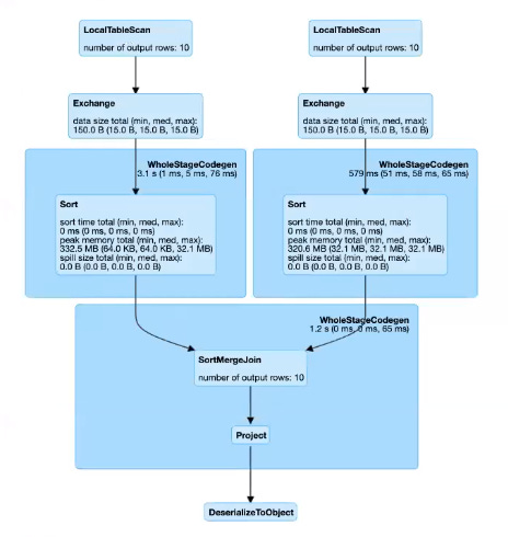
Execution details
Sort-Merge join will span multiple stages in the Spark DAG. Typically, you’ll have one stage (or stages) to produce the shuffle partitions for side A, another for side B, and then a final stage where the actual join (merge) happens. In Spark UI’s DAG visualization, you might see something like: both tables read in earlier stages, then a stage where “Exchange -> Sort -> WholeStageCodegen -> SortMergeJoin” occurs
")
A Spark DAG visualization of a Sort-Merge Join. Both tables are read and then shuffled (Exchange) so that matching keys co-locate. Each partition then sorts its chunk of data on the join key and merges the two sorted streams to output joined rows. (Some upstream stages show as “skipped” because their output was cached for reuse in this example.)
Supported join types: All join types are supported by SMJ for equality conditions – inner, left, right, full outer, semi, anti. It’s the fallback for any join that can’t use a more specialized strategy. Even non-equi joins (like inequalities) can be executed with a sort-merge-like approach if one side is small (Spark might use a Broadcast NLJ for those), but typically equi-joins are where SMJ is used. If you have a full outer join or if both sides are huge, SMJ is usually the plan Spark will choose. (Full outer join cannot be executed as a pure hash join in Spark 2.x, so SMJ was the only choice; Spark 3.1 introduced a shuffle hash algorithm for full outer, but SMJ is still often used.)
Why is it the most stable join?
Sort-Merge Join is network and CPU intensive. It performs a full shuffle of both datasets – which means network I/O proportional to the data size – and a sort of each partition. The memory usage during the sort phase can be high; Spark uses external sort which will spill to disk if a partition’s data doesn’t fit in memory. Unlike SHJ, SMJ is not all-or-nothing in memory: if a task has more data than RAM, it will write sorted runs to disk and merge them (graceful degradation).
This is why SMJ is considered stable for large data – it won’t crash for memory reasons, at worst it will spill and slow down. Still, you want to avoid excessive spilling by tuning partition sizes (Databricks often sets the default shuffle partitions to a high number or uses AQE to auto-tune partition counts).
Because both sides are shuffled, SMJ is symmetric – both large and small tables incur shuffle cost. The algorithm doesn’t build big hash tables, so it can handle very large inputs (even beyond memory) as long as you accept the sorting cost. One positive aspect is that SMJ streaming merge has low overhead per record once sorted, and if data is somewhat presorted or partitioned, the cost might be less than worst-case.
Databricks-specific insights
Databricks Runtime by default enables Adaptive Query Execution (AQE), which can optimize sort-merge joins in two major ways:
Dynamic partition coalescing – after shuffle, if many partitions are small, Databricks can coalesce them to reduce task overhead
Skew handling – if some partitions are extremely large (skewed), Databricks can split those into multiple tasks to avoid stragglers
We will discuss skew handling separately, but it’s important that with AQE, SMJ is not as rigid as it once was. Databricks also collects detailed statistics to decide join strategies: if the optimizer has reliable size estimates (via cost-based optimization), it might avoid SMJ in favor of BHJ when appropriate. However, when dealing with truly large tables where neither side is small, SMJ will be chosen because it’s the most general and robust approach.
Advanced Performance Tuning Strategies
While Spark handles the heavy lifting, you can tune SMJ performance by managing the shuffle and sort behavior:
Partition sizing: Adjust
spark.sql.shuffle.partitionsso that each partition after shuffle is a reasonable size (Databricks often aims for ~128 MB per partition as a balance between parallelism and overhead). Too few partitions (huge partitions) mean slow sorts and potential disk spills; too many (tiny partitions) mean excessive task scheduling overhead. AQE can auto-coalesce partitions that are smaller thanspark.sql.adaptive.advisoryPartitionSizeInBytes(default 64MB)Take advantage of sorting where possible: If your data is bucketed and sorted on the join keys (and both sides have the same number of buckets and join key bucketing), Spark can use a join without shuffle (it still sorts each bucket if not sorted, but avoids data movement). On Databricks, Delta Lake can maintain clustering (Z-order or sorting) on keys; while Spark does not automatically detect sort order for skipping the sort stage, having data clustered can improve CPU cache efficiency during the merge.
Push down filters and projections: Reduce data size before the join. SMJ’s cost is super linear in data volume (due to sorting). If you can filter out unnecessary rows or columns (thus less data to shuffle), do it first. The Catalyst optimizer should push filters, but be mindful when writing queries (e.g., filter as early as possible in the query plan). Also, dropping unused columns means less data is carried through the shuffle.
Monitor for skew: SMJ is particularly vulnerable to skewed keys: if one key accounts for a huge fraction of data, one shuffle partition will be enormous and the merge task for that partition will be a straggler. We’ll discuss skew mitigation soon (Databricks can automatically split skewed partitions. If you suspect skew, the Spark UI’s stage detail can show if one task processed far more data than others.
When to use SMJ
Typically, you don’t force a sort-merge join; Spark will use it by default for large data. But you might choose to use an SMJ (or let Spark use it) in cases where both datasets are large and similar in size, or when you’re doing a full outer join (which BHJ can’t handle). If one side can be broadcast but you choose not to (perhaps due to risk of OOM or because it’s just borderline size), SMJ will handle it gracefully. SMJ is also the strategy that can cope with lack of statistics: if Spark isn’t sure of sizes, it errs on the side of SMJ because it won’t blow up memory. On Databricks, if you disable adaptive execution or broadcasting, you are essentially forcing SMJ for all joins.
Common Pitfalls
Inadequate shuffle partition tuning, leading to excessive disk spills or overhead from numerous tiny partitions.
Failure to minimize shuffle volume by removing unnecessary columns.
Ignoring or inadequately handling data skew.
Misjudging broadcast opportunities by incorrectly assessing dataset size (rely on in-memory exchange size, not disk size).
Pitfalls: The major downside of SMJ is performance degradation if not tuned. Mistakes include not accounting for data skew (leading to very slow tasks) and leaving the default shuffle partitions at 200 regardless of data scale. For instance, joining two 1 TB tables with 200 partitions would create ~5 GB partitions, likely causing massive spills; increasing partitions (or using AQE) would be necessary. Another common pitfall is forgetting that all columns of both sides are shuffled by default. Projecting out unneeded columns can make a huge difference in shuffle volume. Also, if you have multiple joins in a single query (like joining 3-4 tables), Spark might form a multi-way join plan – consider breaking a very large join into steps or using broadcasts for some legs to avoid an overly expensive single SMJ of many inputs.
Conclusion
Sort-Merge Join remains a foundational element in Spark's join strategies. Understanding its detailed mechanics—shuffle, sort, and merge phases. With careful tuning and vigilant analysis, SMJ can transform demanding Spark workloads into highly optimized, reliable operations. On Databricks, always keep AQE enabled for SMJ – it will automatically optimize partition counts and handle skew, making SMJ perform much better in practice than the static execution plans of the past.
Further Resources
Apache Spark Official Documentation – SQL Performance Tuning: Covers join strategy hints, adaptive execution, etc. (See “Join Strategy Hints” and “Adaptive Query Execution” in the Spark docs)
Tuning Spark SQL queries for AWS Glue and Amazon EMR Spark jobs
Apache Spark Official Documentation – Adaptive Query Execution (AQE): Detailed explanation of AQE features like converting SMJ to BHJ/SHJ and skew join handling
Databricks Documentation – Join Hints & Optimizations: Databricks-specific docs on join strategies, including the
SKEWandRANGEhints, and how AQE is used on Databricks“How Databricks Optimizes Spark SQL Joins” – Medium (dezimaldata): A blog post (Aug 2023) summarizing Databricks’ techniques like CBO, AQE, range join and skew join optimizations
Spark Summit Talks on Joins and AQE: Videos like “Optimizing Shuffle Heavy Workloads” or “AQE in Spark 3.0” (by Databricks engineers) for a deeper understanding of the internals of join execution and tuning.
https://spark.apache.org/docs/latest/sql-performance-tuning.html#join-strategy-hints
https://spark.apache.org/docs/latest/sql-performance-tuning.html#adaptive-query-execution
Top 5 Mistakes That Make Your Databricks Queries Slow (and How to Fix Them)


